Contrastive Methods in Energy-Based Models

Recap

Dr. LeCun spent the first ~15 min giving a review of energy-based models. Please refer back to last week (Week 7 notes) for this information, especially the concept of contrastive learning methods.

As we have learned from the last lecture, there are two main classes of learning methods:

1. Contrastive Methods that push down the energy of training data points, $F(x_i, y_i)$, while pushing up energy on everywhere else, $F(x_i, y’)$.
2. Architectural Methods that build energy function $F$ which has minimized/limited low energy regions by applying regularization.

To distinguish the characteristics of different training methods, Dr. Yann LeCun has further summarized 7 strategies of training from the two classes mention before. One of which is methods that are similar to Maximum Likelihood method, which push down the energy of data points and push up everywhere else.

Maximum Likelihood method probabilistically pushes down energies at training data points and pushes everywhere else for every other value of $y’\neq y_i$. Maximum Likelihood doesn’t “care” about the absolute values of energies but only “cares” about the difference between energy. Because the probability distribution is always normalized to sum/integrate to 1, comparing the ratio between any two given data points is more useful than simply comparing absolute values.

Contrastive methods in self-supervised learning

In contrastive methods, we push down on the energy of observed training data points ($x_i$, $y_i$), while pushing up on the energy of points outside of the training data manifold.

In self-supervised learning, we use one part of the input to predict the other parts. We hope that our model can produce good features for computer vision that rival those from supervised tasks.

Researchers have found empirically that applying contrastive embedding methods to self-supervised learning models can indeed have good performances which rival that of supervised models. We will explore some of these methods and their results below.

Contrastive embedding

Consider a pair ($x$, $y$), such that $x$ is an image and $y$ is a transformation of $x$ that preserves its content (rotation, magnification, cropping, etc.). We call this a positive pair.

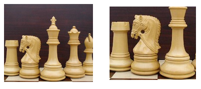
Fig. 1: Positive Pair

Conceptually, contrastive embedding methods take a convolutional network, and feed $x$ and $y$ through this network to obtain two feature vectors: $h$ and $h’$. Because $x$ and $y$ have the same content (i.e. a positive pair), we want their feature vectors to be as similar as possible. As a result, we choose a similarity metric (such as cosine similarity) and a loss function that maximizes the similarity between $h$ and $h’$. By doing this, we lower the energy for images on the training data manifold.

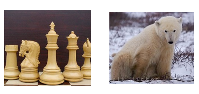
Fig. 2: Negative Pair

However, we also have to push up on the energy of points outside this manifold. So we also generate negative samples ($x_{\text{neg}}$, $y_{\text{neg}}$), images with different content (different class labels, for example). We feed these to our network above, obtain feature vectors $h$ and $h’$, and now try to minimize the similarity between them.

This method allows us to push down on the energy of similar pairs while pushing up on the energy of dissimilar pairs.

Recent results (on ImageNet) have shown that this method can produce features that are good for object recognition that can rival the features learned through supervised methods.

Self-Supervised Results (MoCo, PIRL, SimCLR)

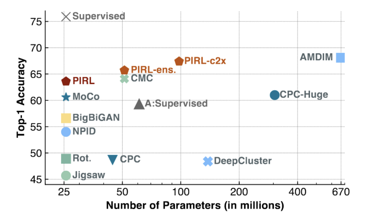
Fig. 3: PIRL and MoCo on ImageNet

As seen in the figure above, MoCo and PIRL achieve SOTA results (especially for lower-capacity models, with a small number of parameters). PIRL is starting to approach the top-1 linear accuracy of supervised baselines (~75%).

We can understand PIRL more by looking at its objective function: NCE (Noise Contrastive Estimator) as follows.

Here we define the similarity metric between two feature maps/vectors as the cosine similarity.

What PIRL does differently is that it doesn’t use the direct output of the convolutional feature extractor. It instead defines different heads $f$ and $g$, which can be thought of as independent layers on top of the base convolutional feature extractor.

Putting everything together, PIRL’s NCE objective function works as follows. In a mini-batch, we will have one positive (similar) pair and many negative (dissimilar) pairs. We then compute the similarity between the transformed image’s feature vector ($I^t$) and the rest of the feature vectors in the minibatch (one positive, the rest negative). We then compute the score of a softmax-like function on the positive pair. Maximizing a softmax score means minimizing the rest of the scores, which is exactly what we want for an energy-based model. The final loss function, therefore, allows us to build a model that pushes the energy down on similar pairs while pushing it up on dissimilar pairs.

Dr. LeCun mentions that to make this work, it requires a large number of negative samples. In SGD, it can be difficult to consistently maintain a large number of these negative samples from mini-batches. Therefore, PIRL also uses a cached memory bank.

Question: Why do we use cosine similarity instead of L2 Norm? Answer: With an L2 norm, it’s very easy to make two vectors similar by making them “short” (close to centre) or make two vectors dissimilar by making them very “long” (away from the centre). This is because the L2 norm is just a sum of squared partial differences between the vectors. Thus, using cosine similarity forces the system to find a good solution without “cheating” by making vectors short or long.

SimCLR

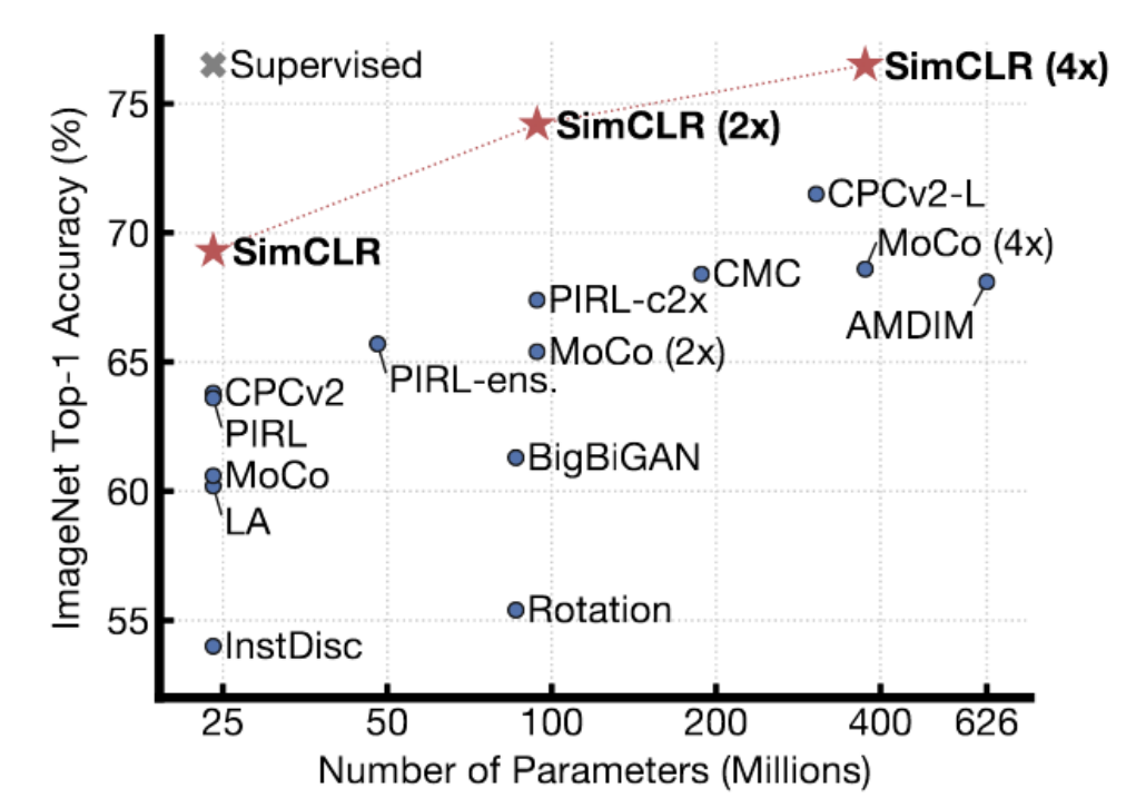
Fig. 4: SimCLR Results on ImageNet

SimCLR shows better results than previous methods. In fact, it reaches the performance of supervised methods on ImageNet, with top-1 linear accuracy on ImageNet. The technique uses a sophisticated data augmentation method to generate similar pairs, and they train for a massive amount of time (with very, very large batch sizes) on TPUs. Dr. LeCun believes that SimCLR, to a certain extent, shows the limit of contrastive methods. There are many, many regions in a high-dimensional space where you need to push up the energy to make sure it’s actually higher than on the data manifold. As you increase the dimension of the representation, you need more and more negative samples to make sure the energy is higher in those places not on the manifold.

Denoising autoencoder

In week 7’s practicum, we discussed denoising autoencoder. The model tends to learn the representation of the data by reconstructing corrupted input to the original input. More specifically, we train the system to produce an energy function that grows quadratically as the corrupted data move away from the data manifold.

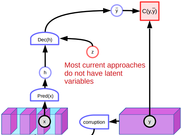
Fig. 5: Architecture of denoising autoencoder

Issues

However, there are several problems with denoising autoencoders. One problem is that in a high dimensional continuous space, there are uncountable ways to corrupt a piece of data. So there is no guarantee that we can shape the energy function by simply pushing up on lots of different locations. Another problem with the model is that it performs poorly when dealing with images due to the lack of latent variables. Since there are many ways to reconstruct the images, the system produces various predictions and doesn’t learn particularly good features. Besides, corrupted points in the middle of the manifold could be reconstructed to both sides. This will create flat spots in the energy function and affect the overall performance.

Other Contrastive Methods

There are other contrastive methods such as contrastive divergence, Ratio Matching, Noise Contrastive Estimation, and Minimum Probability Flow. We will briefly discuss the basic idea of contrastive divergence.

Contrastive Divergence

Contrastive divergence (CD) is another model that learns the representation by smartly corrupting the input sample. In a continuous space, we first pick a training sample $y$ and lower its energy. For that sample, we use some sort of gradient-based process to move down on the energy surface with noise. If the input space is discrete, we can instead perturb the training sample randomly to modify the energy. If the energy we get is lower, we keep it. Otherwise, we discard it with some probability. Keep doing so will eventually lower the energy of $y$. We can then update the parameter of our energy function by comparing $y$ and the contrasted sample $\bar y$ with some loss function.

Persistent Contrastive Divergence

One of the refinements of contrastive divergence is persistent contrastive divergence. The system uses a bunch of “particles” and remembers their positions. These particles are moved down on the energy surface just like what we did in the regular CD. Eventually, they will find low energy places in our energy surface and will cause them to be pushed up. However, the system does not scale well as the dimensionality increases.