Generative Adversarial Networks

Introduction to generative adversarial networks (GANs)

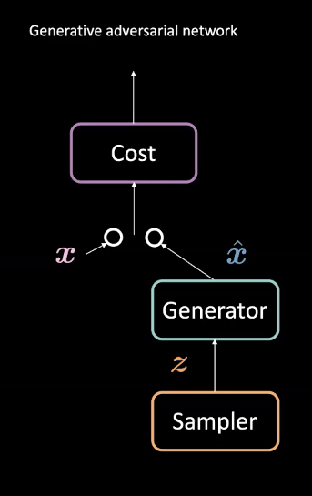
Fig. 1: GAN Architecture

GANs are a type of neural network used for unsupervised machine learning. They are comprised of two adversarial modules: generator and cost networks. These modules compete with each other such that the cost network tries to filter fake examples while the generator tries to trick this filter by creating realistic examples $\vect{\hat{x}}$. Through this competition, the model learns a generator that creates realistic data. They can be used in tasks such as future predictions or for generating images after being trained on a particular dataset.

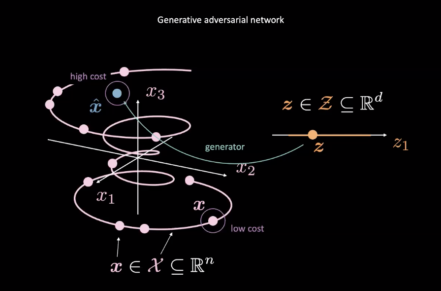
Fig. 2: GAN Mapping from Random Variable

GANs are examples of energy based models (EBMs). As such, the cost network is trained to produce low costs for inputs closer to the true data distribution denoted by the pink $\vect{x}$ in Fig. 2. Data from other distributions, like the blue $\vect{\hat{x}}$ in Fig. 2, should have high cost. A mean squared error (MSE) loss is typically used to calculate the cost network’s performance. It is worth noting that the cost function outputs a positive scalar value within a specified range i.e.$\text{cost} : \mathbb{R}^n \rightarrow \mathbb{R}^+ \cup {0}$). This is unlike a classic discriminator which uses discrete classification for its outputs.

Meanwhile, the generator network ($\text{generator} : \mathcal{Z} \rightarrow \mathbb{R}^n$) is trained to improve its mapping of random variable $\vect{z}$ to realistic generated data $\vect{\hat{x}}$ to trick the cost network. The generator is trained with respect to the cost network’s output, trying to minimize the energy of $\vect{\hat{x}}$. We denote this energy as $C(G(\vect{z}))$, where $C(\cdot)$ is the cost network and $G(\cdot)$ is the generator network.

The training of the cost network is based on minimizing the MSE loss, while the training of the generator network is through minimizing the cost network, using gradients of $C(\vect{\hat{x}})$ with respect to $\vect{\hat{x}}$.

To ensure that high cost is assigned to points outside the data manifold and low cost is assigned to points within it, the loss function for the cost network $\mathcal{L}_{C}$ is $C(x)+[m-C(G(\vect{z}))]^+$ for some positive margin $m$. Minimizing $\mathcal{L}_{C}$ requires that $C(\vect{x}) \rightarrow 0$ and $C(G(\vect{z})) \rightarrow m$. The loss for the generator $\mathcal{L}_{G}$ is simply $C(G(\vect{z}))$, which encourages the generator to ensure that $C(G(\vect{z})) \rightarrow 0$. However, this does create instability as $0 \leftarrow C(G(\vect{z})) \rightarrow m$.

Difference between GANs and VAEs

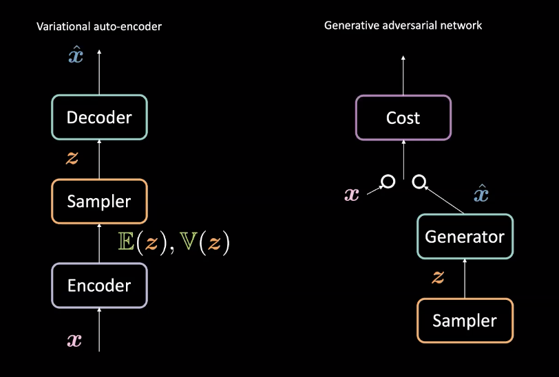
Fig. 3: VAE (left) *vs.* GAN (right) - Architectural design

Compared to Variational Auto-Encoders (VAEs) from week 8, GANs create generators slightly differently. Recall, VAEs map inputs $\vect{x}$ to a latent space $\mathcal{Z}$ with an encoder and then map from $\mathcal{Z}$ back to the data space with a decoder to get $\vect{\hat{x}}$. They then use the reconstruction loss to push $\vect{x}$ and $\vect{\hat{x}}$ to be similar. GANs, on the other hand, train through an adversarial setting with the generator and cost networks competing as described above. These networks are successively trained through backpropagation through gradient based methods. Comparison of this architectural difference can be seen in Fig. 3.

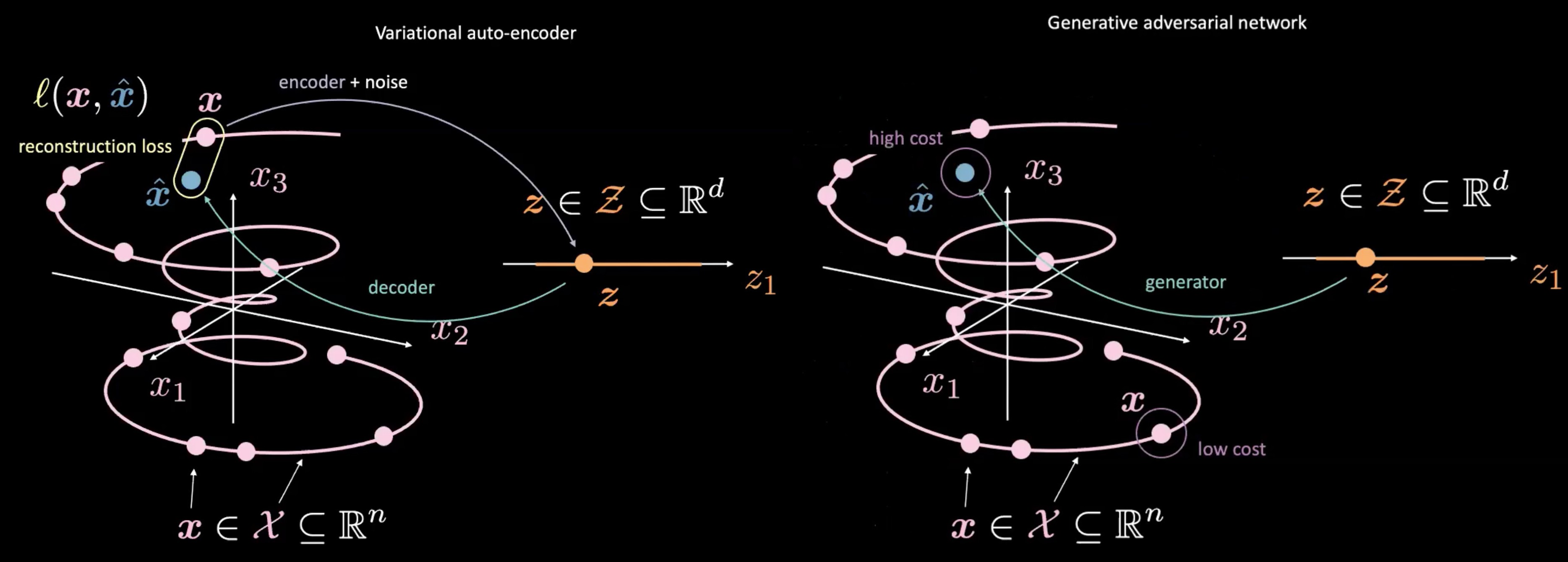
Fig. 4: VAE (left) *vs.* GAN (right) - Mapping from Random Sample $\vect{z}$

GANs also differ from VAEs through how they produce and use $\vect{z}$. GANs start by sampling $\vect{z}$, similar to the latent space in a VAE. They then use a generative network to map $\vect{z}$ to $\vect{\hat{x}}$. This $\vect{\hat{x}}$ is then sent through a discriminator/cost network to evaluate how “real” it is. One of the main differences from VAE and GAN is that we do not need to measure a direct relationship (i.e. reconstruction loss) between the output of the generative network $\vect{\hat{x}}$ and real data $\vect{x}$. Instead, we force $\vect{\hat{x}}$ to be similar to $\vect{x}$ by training the generator to produce $\vect{\hat{x}}$ such that the discriminator/cost network produces scores that are similar to those of real data $\vect{x}$, or more “real”.

Major pitfalls in GANs

While GANs can be powerful for building generators, they have some major pitfalls.

1. Unstable convergence

As the generator improves with training, the discriminator performance gets worse because the discriminator can no longer easily tell the difference between real and fake data. If the generator is perfect, then the manifold of the real and fake data will lie on top of each other and the discriminator will create many misclassifications.

This poses a problem for convergence of the GAN: the discriminator feedback gets less meaningful over time. If the GAN continues training past the point when the discriminator is giving completely random feedback, then the generator starts to train on junk feedback and its quality may collapse. [Refer to training convergence in GANs]

As a result of this adversarial nature between the generator and discriminator there is an unstable equilibrium point rather than an equilibrium.

2. Vanishing gradient

Let’s consider using the binary cross entropy loss for a GAN:

As the discriminator becomes more confident, $D(\vect{x})$ gets closer to $1$ and $D(\vect{\hat{x}})$ gets closer to $0$. This confidence moves the outputs of the cost network into flatter regions where the gradients become more saturated. These flatter regions provide small, vanishing gradients that hinder the generator network’s training. Thus, when training a GAN, you want to make sure that the cost gradually increases as you become more confident.

3. Mode collapse

If a generator maps all $\vect{z}$’s from the sampler to a single $\vect{\hat{x}}$ that can fool the discriminator, then the generator will produce only that $\vect{\hat{x}}$. Eventually, the discriminator will learn to detect specifically this fake input. As a result, the generator simply finds the next most plausible $\vect{\hat{x}}$ and the cycle continues. Consequently, the discriminator gets trapped in local minima while cycling through fake $\vect{\hat{x}}$’s. A possible solution to this issue is to enforce some penalty to the generator for always giving the same output given different inputs.

Deep Convolutional Generative Adversarial Network (DCGAN) source code

The source code of the example can be found here.

Generator

1. The generator upsamples the input using several nn.ConvTranspose2d modules separated with nn.BatchNorm2d and nn.ReLU.
2. At the end of the sequential, the network uses nn.Tanh() to squash outputs to $(-1,1)$.
3. The input random vector has size $nz$. The output has size $nc \times 64 \times 64$, where $nc$ is the number of channels.

class Generator(nn.Module):
    def __init__(self):
        super().__init__()
        self.main = nn.Sequential(
            # input is Z, going into a convolution
            nn.ConvTranspose2d(     nz, ngf * 8, 4, 1, 0, bias=False),
            nn.BatchNorm2d(ngf * 8),
            nn.ReLU(True),
            # state size. (ngf*8) x 4 x 4
            nn.ConvTranspose2d(ngf * 8, ngf * 4, 4, 2, 1, bias=False),
            nn.BatchNorm2d(ngf * 4),
            nn.ReLU(True),
            # state size. (ngf*4) x 8 x 8
            nn.ConvTranspose2d(ngf * 4, ngf * 2, 4, 2, 1, bias=False),
            nn.BatchNorm2d(ngf * 2),
            nn.ReLU(True),
            # state size. (ngf*2) x 16 x 16
            nn.ConvTranspose2d(ngf * 2,     ngf, 4, 2, 1, bias=False),
            nn.BatchNorm2d(ngf),
            nn.ReLU(True),
            # state size. (ngf) x 32 x 32
            nn.ConvTranspose2d(    ngf,      nc, 4, 2, 1, bias=False),
            nn.Tanh()
            # state size. (nc) x 64 x 64
        )

    def forward(self, input):
        output = self.main(input)
        return output

Discriminator

1. It is important to use nn.LeakyReLU as the activation function to avoid killing the gradients in negative regions. Without these gradients, the generator will not receive updates.
2. At the end of the sequential, the discriminator uses nn.Sigmoid() to classify the input.

class Discriminator(nn.Module):
    def __init__(self):
        super().__init__()
        self.main = nn.Sequential(
            # input is (nc) x 64 x 64
            nn.Conv2d(nc, ndf, 4, 2, 1, bias=False),
            nn.LeakyReLU(0.2, inplace=True),
            # state size. (ndf) x 32 x 32
            nn.Conv2d(ndf, ndf * 2, 4, 2, 1, bias=False),
            nn.BatchNorm2d(ndf * 2),
            nn.LeakyReLU(0.2, inplace=True),
            # state size. (ndf*2) x 16 x 16
            nn.Conv2d(ndf * 2, ndf * 4, 4, 2, 1, bias=False),
            nn.BatchNorm2d(ndf * 4),
            nn.LeakyReLU(0.2, inplace=True),
            # state size. (ndf*4) x 8 x 8
            nn.Conv2d(ndf * 4, ndf * 8, 4, 2, 1, bias=False),
            nn.BatchNorm2d(ndf * 8),
            nn.LeakyReLU(0.2, inplace=True),
            # state size. (ndf*8) x 4 x 4
            nn.Conv2d(ndf * 8, 1, 4, 1, 0, bias=False),
            nn.Sigmoid()
        )

    def forward(self, input):
        output = self.main(input)
        return output.view(-1, 1).squeeze(1)

These two classes are initialized as netG and netD.

Loss function for GAN

We use Binary Cross Entropy (BCE) between target and output.

criterion = nn.BCELoss()

Setup

We set up fixed_noise of size opt.batchSize and length of random vector nz. We also create labels for real data and generated (fake) data called real_label and fake_label, respectively.

fixed_noise = torch.randn(opt.batchSize, nz, 1, 1, device=device)
real_label = 1
fake_label = 0

Then we set up optimizers for discriminator and generator networks.

optimizerD = optim.Adam(netD.parameters(), lr=opt.lr, betas=(opt.beta1, 0.999))
optimizerG = optim.Adam(netG.parameters(), lr=opt.lr, betas=(opt.beta1, 0.999))

Training

Each epoch of training is divided into two steps.

Step 1 is to update the discriminator network. This is done in two parts. First, we feed the discriminator real data coming from dataloaders, compute the loss between the output and real_label, and then accumulate gradients with backpropagation. Second, we feed the discriminator data generated by the generator network using the fixed_noise, compute the loss between the output and fake_label, and then accumulate the gradient. Finally, we use the accumulated gradients to update the parameters for the discriminator network.

Note that we detach the fake data to stop gradients from propagating to the generator while we train the discriminator.

Also note that we only need to call zero_grad() once in the beginning to clear the gradients so the gradients from both the real and fake data can be used for the update. The two .backward() calls accumulate these gradients. We finally only need one call of optimizerD.step() to update the parameters.

# train with real
netD.zero_grad()
real_cpu = data[0].to(device)
batch_size = real_cpu.size(0)
label = torch.full((batch_size,), real_label, device=device)

output = netD(real_cpu)
errD_real = criterion(output, label)
errD_real.backward()
D_x = output.mean().item()

# train with fake
noise = torch.randn(batch_size, nz, 1, 1, device=device)
fake = netG(noise)
label.fill_(fake_label)
output = netD(fake.detach())
errD_fake = criterion(output, label)
errD_fake.backward()
D_G_z1 = output.mean().item()
errD = errD_real + errD_fake
optimizerD.step()

Step 2 is to update the Generator network. This time, we feed the discriminator the fake data, but compute the loss with the real_label! The purpose of doing this is to train the generator to make realistic $\vect{\hat{x}}$’s.

netG.zero_grad()
label.fill_(real_label)  # fake labels are real for generator cost
output = netD(fake)
errG = criterion(output, label)
errG.backward()
D_G_z2 = output.mean().item()
optimizerG.step()