Applications of Convolutional Network

Zip Code Recognition

In the previous lecture, we demonstrated that a convolutional network can recognize digits, however, the question remains, how does the model pick each digit and avoid perturbation on neighboring digits. The next step is to detect non/overlapping objects and use the general approach of Non-Maximum Suppression (NMS). Now, given the assumption that the input is a series of non-overlapping digits, the strategy is to train several convolutional networks and using either majority vote or picking the digits corresponding to the highest score generated by the convolutional network.

Recognition with CNN

Here we present the task of recognizing 5 non-overlapping zip codes. The system was not given any instructions on how to separate each digit but knows that is must predict 5 digits. The system (Figure 1) consists of 4 different sized convolutional networks, each producing one set of outputs. The output is represented in matrices. The four output matrices are from models with a different kernel width in the last layer. In each output, there are 10 rows, representing 10 categories from 0 to 9. The larger white square represents a higher score in that category. In these four output blocks, the horizontal sizes of the last kernel layers are 5, 4, 3 and 2 respectively. The size of the kernel decides the width of the model’s viewing window on the input, therefore each model is predicting digits based on different window sizes. The model then takes a majority vote and selects the category that corresponds to the highest score in that window. To extract useful information, one should keep in mind that not all combinations of characters are possible, therefore error correction leveraging input restrictions is useful to ensure the outputs are true zip codes.

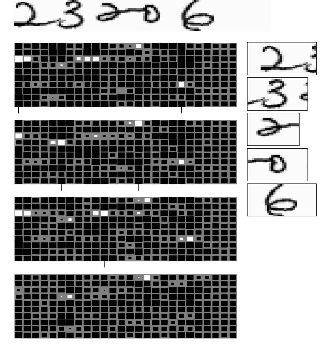
Figure 1: Multiple classifiers on zip code recognition

Now to impose the order of the characters. The trick is to utilize a shortest path algorithm. Since we are given ranges of possible characters and the total number of digits to predict, We can approach this problem by computing the minimum cost of producing digits and transitions between digit. The path has to be continuous from the lower left cell to the upper right cell on the graph, and the path is restricted to only contain movements from left to right and bottom to top. Note that if the same number is repeated next to each other, the algorithm should be able to distinguish there are repeated numbers instead of predicting a single digit.

Face detection

Convolutional neural networks perform well on detection tasks and face detection is no exception. To perform face detection we collect a dataset of images with faces and without faces, on which we train a convolutional net with a window size such as 30 $\times$ 30 pixels and ask the network to tell whether there is a face or not. Once trained, we apply the model to a new image and if there are faces roughly within a 30 $\times$ 30 pixel window, the convolutional net will light up the output at the corresponding locations. However, two problems exist.

• False Positives: There are many different variations of non-face objects that may appear in a patch of an image. During the training stage, the model may not see all of them (i.e. a fully representative set of non-face patches). Therefore, the model may suffer from a lot of false positives at test time. For example, if the network has not been trained on images containing hands, it may detect faces based on skin tones and incorrectly classify patches of images containing hands as faces, thereby giving rise to false positives.

• Different Face Size: Not all faces are 30 $\times$ 30 pixels, so faces of differing sizes may not be detected. One way to handle this issue is to generate multi-scale versions of the same image. The original detector will detect faces around 30 $\times$ 30 pixels. If applying a scale on the image of factor $\sqrt 2$, the model will detect faces that were smaller in the original image since what was 30 $\times$ 30 is now 20 $\times$ 20 pixels roughly. To detect bigger faces, we can downsize the image. This process is inexpensive as half of the expense comes from processing the original non-scaled image. The sum of the expenses of all other networks combined is about the same as processing the original non-scaled image. The size of the network is the square of the size of the image on one side, so if you scale down the image by $\sqrt 2$, the network you need to run is smaller by a factor of 2. So the overall cost is $1+1/2+1/4+1/8+1/16…$, which is 2. Performing a multi-scale model only doubles the computational cost.

A multi-scale face detection system

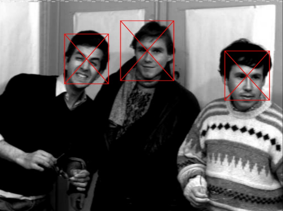
Figure 2: Face detection system

The maps shown in (Figure 3) indicate the scores of face detectors. This face detector recognizes faces that are 20 $\times$ 20 pixels in size. In fine-scale (Scale 3) there are many high scores but are not very definitive. When the scaling factor goes up (Scale 6), we see more clustered white regions. Those white regions represent detected faces. We then apply non-maximum suppression to get the final location of the face.

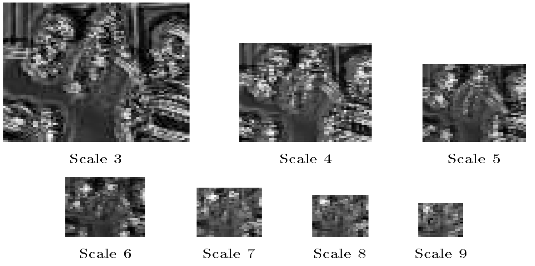
Figure 3: Face detector scores for various scaling factors

Non-maximum suppression

For each high-scoring region, there is probably a face underneath. If more faces are detected very close to the first, it means that only one should be considered correct and the rest are wrong. With non-maximum suppression, we take the highest-scoring of the overlapping bounding boxes and remove the others. The result will be a single bounding box at the optimum location.

Negative mining

In the last section, we discussed how the model may run into a large number of false positives at test time as there are many ways for non-face objects to appear similar to a face. No training set will include all the possible non-face objects that look like faces. We can mitigate this problem through negative mining. In negative mining, we create a negative dataset of non-face patches which the model has (erroneously) detected as faces. The data is collected by running the model on inputs that are known to contain no faces. Then we retrain the detector using the negative dataset. We can repeat this process to increase the robustness of our model against false positives.

Semantic segmentation

Semantic segmentation is the task of assigning a category to every pixel in an input image.

CNN for Long Range Adaptive Robot Vision

In this project, the goal was to label regions from input images so that a robot can distinguish between roads and obstacles. In the figure, the green regions are areas the robot can drive on and the red regions are obstacles like tall grass. To train the network for this task, we took a patch from the image and manually label it traversable or not (green or red). We then train the convolutional network on the patches by asking it to predict the color of the patch. Once the system is sufficiently trained, it is applied to the entire image, labeling all the regions of the image as green or red.

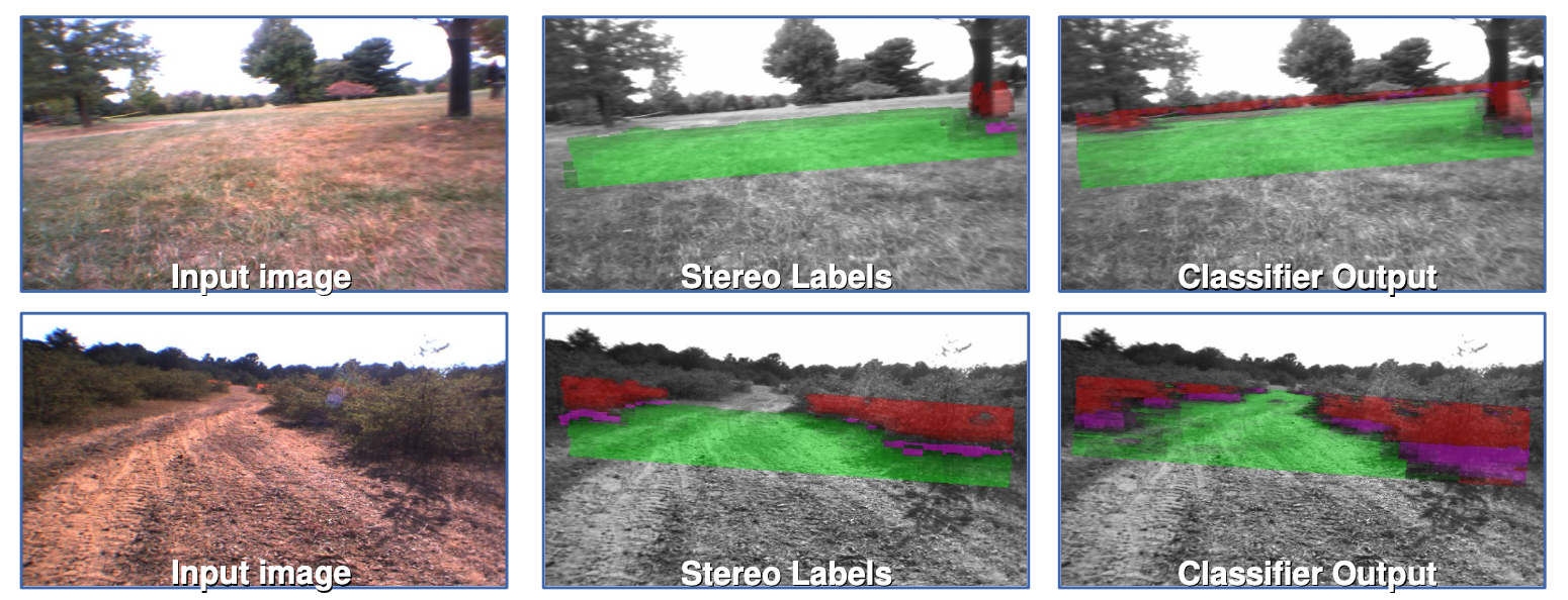
Figure 4: CNN for Long Range Adaptive Robot Vision (DARPA LAGR program 2005-2008)

There were five categories for prediction: 1) super green, 2) green, 3) purple: obstacle foot line, 4) red obstacle 5) super red: definitely an obstacle.

Stereo Labels (Figure 4, Column 2) Images are captured by the 4 cameras on the robot, which are grouped into 2 stereo vision pairs. Using the known distances between the stereo pair cameras, the positions of every pixel in 3D space are then estimated by measuring the relative distances between the pixels that appear in both the cameras in a stereo pair. This is the same process our brains use to estimate the distance of the objects that we see. Using the estimated position information, a plane is fit to the ground, and pixels are then labeled as green if they are near the ground and red if they are above it.

• Limitations & Motivation for ConvNet: The stereo vision only works up to 10 meters and driving a robot requires long-range vision. A ConvNet however, is capable of detecting objects at much greater distances, if trained correctly.

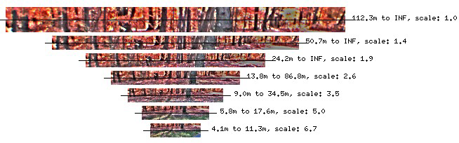
Figure 5: Scale-invariant Pyramid of Distance-normalized Images

• Served as Model Inputs: Important pre-processing includes building a scale-invariant pyramid of distance-normalized images (Figure 5). It is similar to what we have done earlier of this lecture when we tried to detect faces of multiple scales.

Model Outputs (Figure 4, Column 3)

The model outputs a label for every pixel in the image up to the horizon. These are classifier outputs of a multi-scale convolutional network.

• How the Model Becomes Adaptive: The robots have continuous access to the stereo labels, allowing the network to re-train, adapting to the new environment it’s in. Please note that only the last layer of the network would be re-trained. The previous layers are trained in the lab and fixed.

System Performance

When trying to get to a GPS coordinate on the other side of a barrier, the robot “saw” the barrier from far away and planned a route that avoided it. This is thanks to the CNN detecting objects up 50-100m away.

Limitation

Back in the 2000s, computation resources were restricted. The robot was able to process around 1 frame per second, which means it would not be able to detect a person that walks in its way for a whole second before being able to react. The solution for this limitation is a Low-Cost Visual Odometry model. It is not based on neural networks, has a vision of ~2.5m but reacts quickly.

Scene Parsing and Labelling

In this task, the model outputs an object category (buildings, cars, sky, etc.) for every pixel. The architecture is also multi-scale (Figure 6).

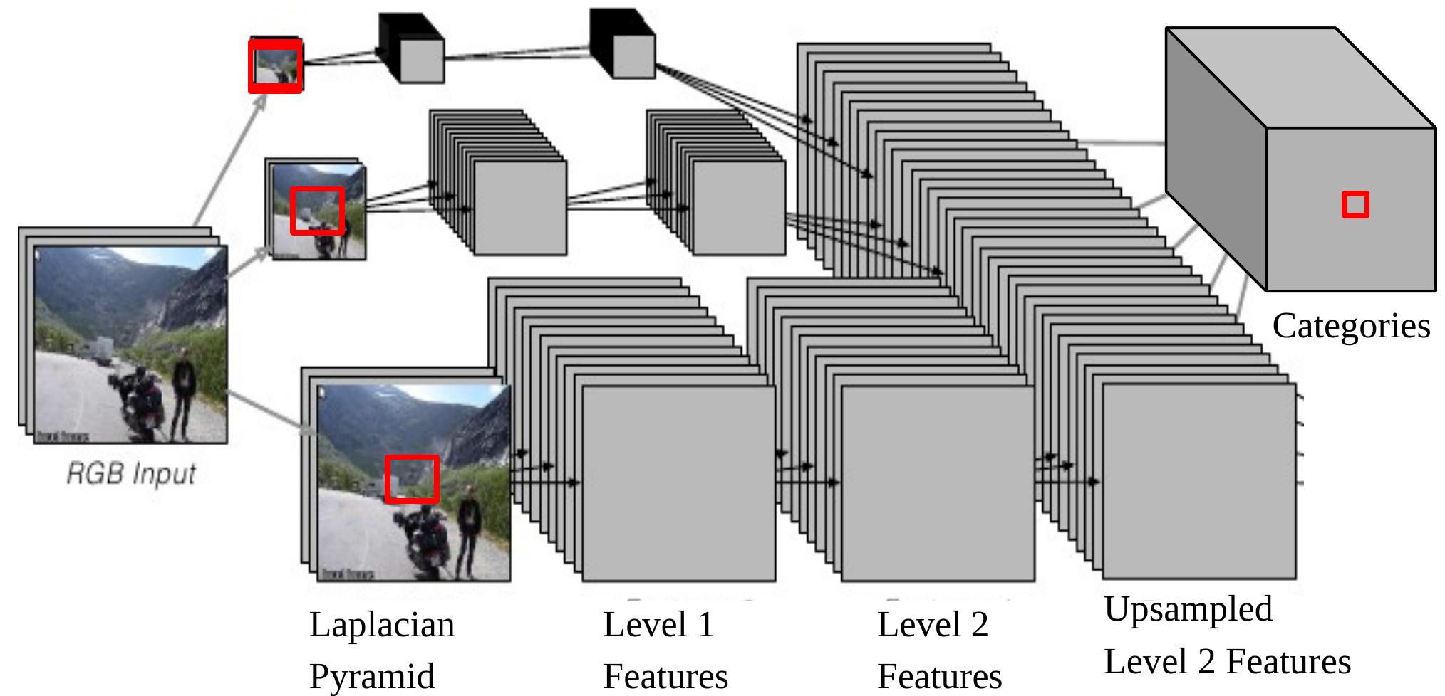
Figure 6: Multi-scale CNN for scene parsing

Notice that if we back project one output of the CNN onto the input, it corresponds to an input window of size $46\times46$ on the original image at the bottom of the Laplacian Pyramid. It means we are using the context of $46\times46$ pixels to decide the category of the central pixel.

However, sometimes this context size is not enough to determine the category for larger objects.

The multiscale approach enables a wider vision by providing extra rescaled images as inputs. The steps are as follows:

1. Take the same image, reduce it by the factor of 2 and a factor of 4, separately.
2. These two extra rescaled images are fed to the same ConvNet (same weights, same kernels) and we get another two sets of Level 2 Features.
3. Upsample these features so that they have the same size as the Level 2 Features of the original image.
4. Stack the three sets of (upsampled) features together and feed them to a classifier.

Now the largest effective size of content, which is from the 1/4 resized image, is $184\times 184\, (46\times 4=184)$.

Performance: With no post-processing and running frame-by-frame, the model runs very fast even on standard hardware. It has a rather small size of training data (2k~3k), but the results are still record-breaking.