Properties of natural signals

Properties of natural signals

All signals can be thought of as vectors. As an example, an audio signal is a 1D signal $\boldsymbol{x} = [x_1, x_2, \cdots, x_T]$ where each value $x_t$ represents the amplitude of the waveform at time $t$. To make sense of what someone is speaking, your cochlea first converts the air pressure vibrations to signals and then your brain uses a language model to convert this signal to a language i.e. it needs to pick the most probable utterance given the signal. For music, the signal is stereophonic which has 2 or more channels to give you an illusion that the sound is coming from multiple directions. Even though it has 2 channels, it’s still a 1D signal because time is the only variable along which the signal is changing.

An image is a 2D signal because the information is spatially depicted. Note that each point can be a vector in itself. This means that if we have $d$ channels in an image, each spatial point in the image is a vector of dimension $d$. A colour image has RGB planes, which means $d = 3$. For any point $x_{i,j}$, this corresponds to the intensity of red, green and blue colours respectively.

We can even represent language with the above logic. Each word corresponds to a one-hot vector with one at the position it occurs in our vocabulary and zeroes everywhere else. This means that each word is a vector of the size of the vocabulary.

Natural data signals follow these properties:

1. Stationarity: Certain motifs repeat throughout a signal. In audio signals, we observe the same type of patterns over and over again across the temporal domain. In images, this means that we can expect similar visual patterns repeat across the dimensionality.
2. Locality: Nearby points are more correlated than points far away. For 1D signal, this means that if we observe a peak at some point $t_i$, we expect the points in a small window around $t_i$ to have similar values as $t_i$ but for a point $t_j$ far away from $t_i$, $x_{t_i}$ has very less bearing on $x_{t_j}$. More formally, the convolution between a signal and its flipped counterpart has a peak when the signal is perfectly overlapping with it’s flipped version. A convolution between two 1D signals (cross-correlation) is nothing but their dot product which is a measure of how similar or close the two vectors are. Thus, information is contained in specific portions and parts of the signal. For images, this means that the correlation between two points in an image decreases as we move the points away. If $x_{0,0}$ pixel is blue, the probability that the next pixel ($x_{1,0},x_{0,1}$) is also blue is pretty high but as you move to the opposite end of the image ($x_{-1,-1}$), the value of this pixel is independent of the pixel value at $x_{0,0}$.
3. Compositionality: Everything in nature is composed of parts that are composed of sub-parts and so on. As an example, characters form strings that form words, which further form sentences. Sentences can be combined to form documents. Compositionality allows the world to be explainable.

If our data exhibits stationarity, locality, and compositionality, we can exploit them with networks that use sparsity, weight sharing and stacking of layers.

Exploiting properties of natural signals to build invariance and equivariance

Locality $\Rightarrow$ sparsity

Fig.1 shows a 5-layer fully connected network. Each arrow represents a weight to be multiplied by the inputs. As we can see, this network is very computationally expensive.

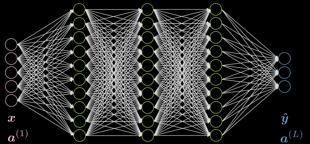
Figure 1: Fully Connected Network

If our data exhibits locality, each neuron needs to be connected to only a few local neurons of the previous layer. Thus, some connections can be dropped as shown in Fig.2. Fig.2(a) represents an FC network. Taking advantage of the locality property of our data, we drop connections between far away neurons in Fig.2(b). Although the hidden layer neurons (green) in Fig.2(b) don’t span the whole input, the overall architecture will be able to account for all input neurons. The receptive field (RF) is the number of neurons of previous layers, that each neuron of a particular layer can see or has taken into account. Therefore, the RF of the output layer w.r.t the hidden layer is 3, RF of the hidden layer w.r.t the input layer is 3, but the RF of the output layer w.r.t the input layer is 5.

Figure 2(a): Before Applying Sparsity	Figure 2(b): After Applying Sparsity

Stationarity $\Rightarrow$ parameters sharing

If our data exhibits stationarity, we could use a small set of parameters multiple times across the network architecture. For example in our sparse network, Fig.3(a), we can use a set of 3 shared parameters (yellow, orange and red). The number of parameters will then drop from 9 to 3! The new architecture might even work better because we have more data for training those specific weights. The weights after applying sparsity and parameter sharing is called a convolution kernel.

Figure 3(a): Before Applying Parameter Sharing	Figure 3(b): After Applying Parameter Sharing

Following are some advantages of using sparsity and parameter sharing:-

• Parameter sharing
  • faster convergence
  • better generalisation
  • not constained to input size
  • kernel indepence $\Rightarrow$ high parallelisation
• Connection sparsity
  • reduced amount of computation

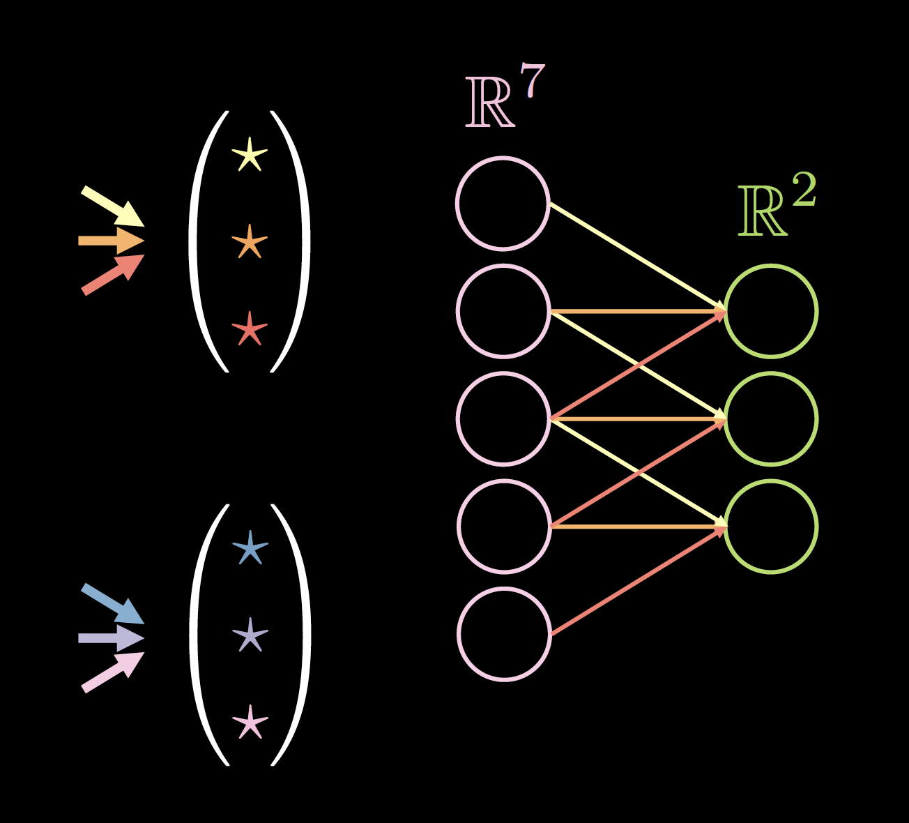
Fig.4 shows an example of kernels on 1D data, where the kernel size is: 2(number of kernels) * 7(thickness of the previous layer) * 3(number of unique connections/weights).

The choice of kernel size is empirical. 3 * 3 convolution seems to be the minimal size for spatial data. Convolution of size 1 can be used to obtain a final layer that can be applied to a larger input image. Kernel size of even number might lower the quality of the data, thus we always have kernel size of odd numbers, usually 3 or 5.

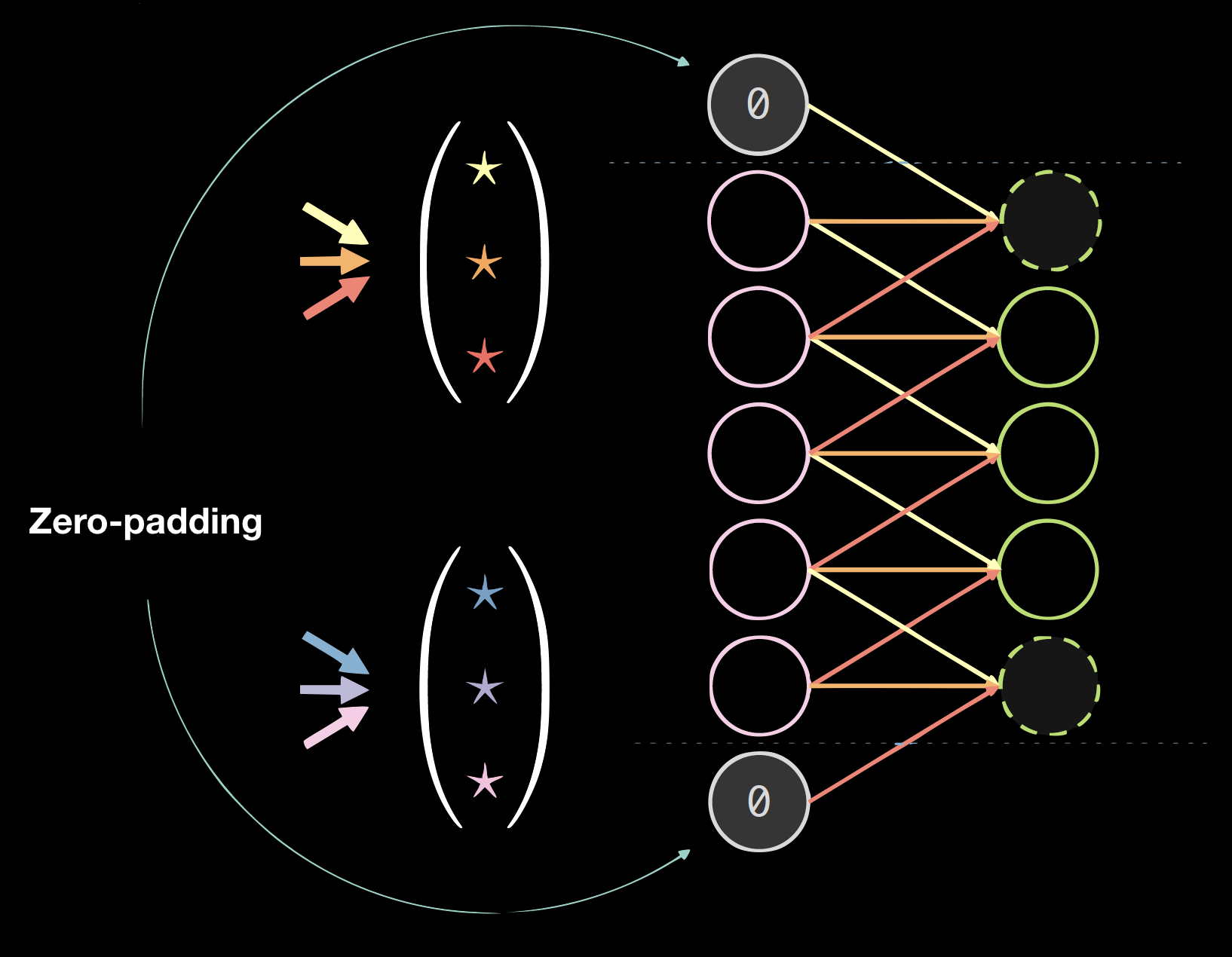Figure 4(a): Kernels on 1D Data	Figure 4(b): Data with Zero Padding

Padding

Padding generally hurts the final results, but it is convenient programmatically. We usually use zero-padding: size = (kernel size - 1)/2.

Standard spatial CNN

A standard spatial CNN has the following properties:

• Multiple layers
  • Convolution
  • Non-linearity (ReLU and Leaky)
  • Pooling
  • Batch normalisation
• Residual bypass connection

Batch normalization and residual bypass connections are very helpful to get the network to train well. Parts of a signal can get lost if too many layers have been stacked so, additional connections via residual bypass, guarantee a path from bottom to top and also for a path for gradients coming from top to bottom.

In Fig.5, while the input image contains mostly spatial information across two dimensions (apart from characteristic information, which is the colour of each pixel), the output layer is thick. Midway, there is a trade off between the spatial information and the characteristic information and the representation becomes denser. Therefore, as we move up the hierarchy, we get denser representation as we lose the spatial information.

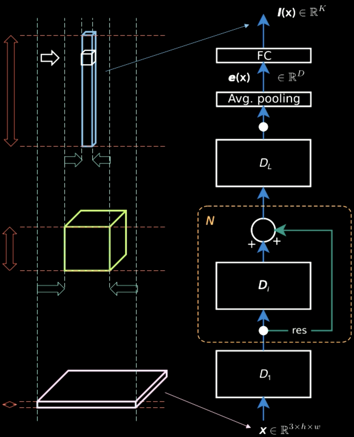
Figure 5: Information Representations Moving up the Hierarchy

Pooling

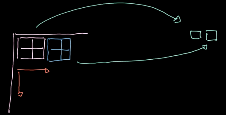
Figure 6: Illustration of Pooling

A specific operator, $L_p$-norm, is applied to different regions (refer to Fig.6). Such an operator gives only one value per region(1 value for 4 pixels in our example). We then iterate over the whole data region-by-region, taking steps based on the stride. If we start with $m * n$ data with $c$ channels, we will end up with $\frac{m}{2} * \frac{n}{2}$ data still with $c$ channels (refer to Fig.7). Pooling is not parametrized; nevertheless, we can choose different polling types like max pooling, average pooling and so on. The main purpose of pooling reduces the amount of data so that we can compute in a reasonable amount of time.

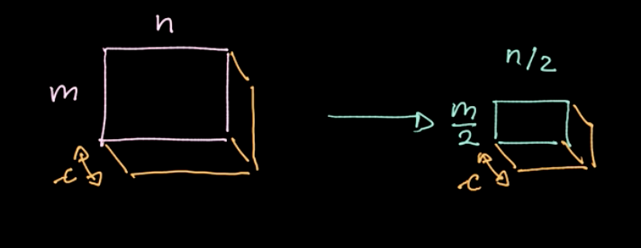
Figure 7: Pooling results

CNN - Jupyter Notebook

The Jupyter notebook can be found here. To run the notebook, make sure you have the pDL environment installed as specified in README.md.

In this notebook, we train a multilayer perceptron (FC network) and a convolution neural network (CNN) for the classification task on the MNIST dataset. Note that both networks have an equal number of parameters. (Fig.8)

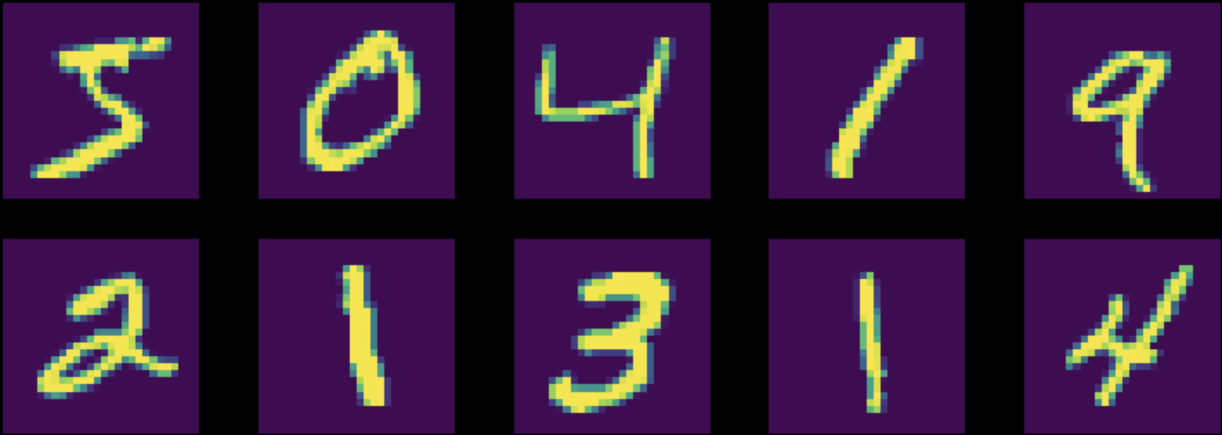
Figure 8: Instances from the Original MNIST Dataset

Before training, we normalize our data so that the initialization of the network will match our data distribution (very important!). Also, make sure that the following five operations/steps are present in your training:

1. Feeding data to the model
2. Computing the loss
3. Cleaning the cache of accumulated gradients with zero_grad()
4. Computing the gradients
5. Performing a step in the optimizer method

First, we train both the networks on the normalized MNIST data. The accuracy of the FC network turned out to be $87\%$ while the accuracy of the CNN turned out to be $95\%$. Given the same number of parameters, the CNN managed to train many more filters. In the FC network, filters that try to get some dependencies between things that are further away with things that are close by, are trained. They are completely wasted. Instead, in the convolutional network, all these parameters concentrate on the relationship between neighbour pixels.

Next, we perform a random permutation of all the pixels in all the images of our MNIST dataset. This transforms our Fig.8 to Fig.9. We then train both the networks on this modified dataset.

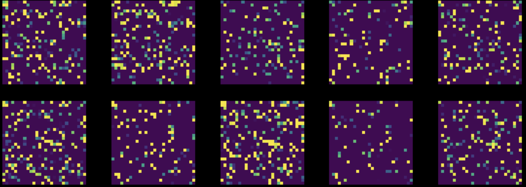
Figure 9: Instances from Permuted MNIST Dataset

The performance of the FC network almost stayed unchanged ($85\%$), but the accuracy of CNN dropped to $83\%$. This is because, after a random permutation, the images no longer hold the three properties of locality, stationarity, and compositionality, that are exploitable by a CNN.