Loss Functions (cont.) and Loss Functions for Energy Based Models

Binary Cross Entropy (BCE) Loss - nn.BCELoss()

This loss is a special case of cross entropy for when you have only two classes so it can be reduced to a simpler function. This is used for measuring the error of a reconstruction in, for example, an auto-encoder. This formula assume $x$ and $y$ are probabilities, so they are strictly between 0 and 1.

Kullback-Leibler Divergence Loss - nn.KLDivLoss()

This is simple loss function for when your target is a one-hot distribution (i.e. $y$ is a category). Again it assumes $x$ and $y$ are probabilities. It has the disadvantage that it is not merged with a softmax or log-softmax so it may have numerical stability issues.

BCE Loss with Logits - nn.BCEWithLogitsLoss()

This version of binary cross entropy loss takes scores that haven’t gone through softmax so it does not assume x is between 0 and 1. It is then passed through a sigmoid to ensure it is in that range. The loss function is more likely to be numerically stable when combined like this.

Margin Ranking Loss - nn.MarginRankingLoss()

Margin losses are an important category of losses. If you have two inputs, this loss function says you want one input to be larger than the other one by at least a margin. In this case $y$ is a binary variable $\in { -1, 1}$. Imagine the two inputs are scores of two categories. You want the score for the correct category larger than the score for the incorrect categories by at least some margin. Like hinge loss, if $y*(x_1-x_2)$ is larger than margin, the cost is 0. If it is smaller, the cost increases linearly. If you were to use this for classification, you would have $x_1$ be the score of the correct answer and $x_2$ be the score of the highest scoring incorrect answer in the mini-batch. If used in energy based models (discussed later), this loss function pushes down on the correct answer $x_1$ and up on the incorrect answer $x_2$.

Triplet Margin Loss - nn.TripletMarginLoss()

This loss is used for measuring a relative similarity between samples. For example, you put two images with the same category through a CNN and get two vectors. You want the distance between those two vectors to be as small as possible. If you put two images with different categories through a CNN, you want the distance between those vectors to be as large as possible. This loss function tries to send the first distance toward 0 and the second distance larger than some margin. However, the only thing that matter is that the distance between the good pair is smaller than the distance between the bad pair.

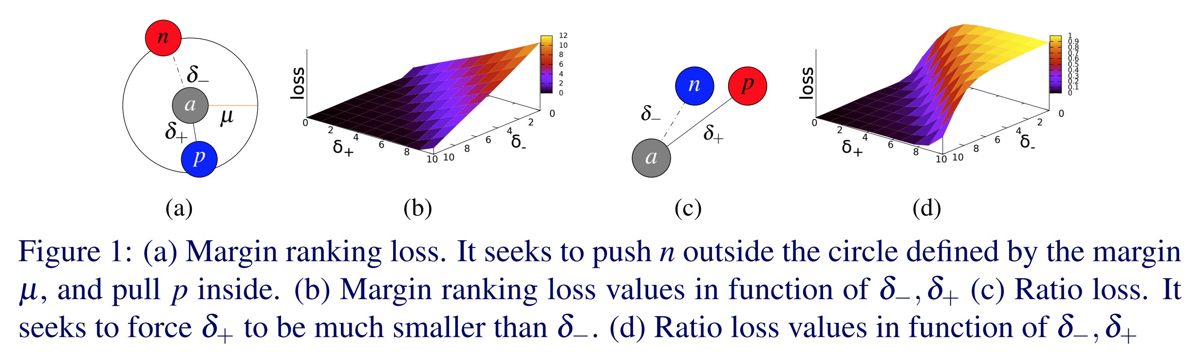
Fig. 1: Triplet Margin Loss

This was originally used to train an image search system for Google. At that time, you would type a query into Google and it would encode that query into a vector. It would then compare that vector to a bunch of vectors from images that were previously indexed. Google would then retrieve the images that were the closest to your vector.

Soft Margin Loss - nn.SoftMarginLoss()

Creates a criterion that optimizes a two-class classification logistic loss between input tensor $x$ and target tensor $y$ (containing 1 or -1).

• This softmax version of a margin loss. You have a bunch of positives and a bunch of negatives you want to pass through a softmax. This loss function then tries to make $\text{exp}(-y[i]*x[i])$ for the correct $x[i]$ smaller than for any other.
• This loss function wants to pull the positive values of $y[i]*x[i]$ closer together and push the negative values far apart but, as opposed to a hard margin, with some continuous, exponentially decaying effect on the loss .

Multi-Class Hinge Loss - nn.MultiLabelMarginLoss()

This margin-base loss allows for different inputs to have variable amounts of targets. In this case you have several categories for which you want high scores and it sums the hinge loss over all categories. For EBMs, this loss function pushes down on desired categories and pushes up on non-desired categories.

Hinge Embedding Loss - nn.HingeEmbeddingLoss()

Hinge embedding loss used for semi-supervised learning by measuring whether two inputs are similar or dissimilar. It pulls together things that are similar and pushes away things are dissimilar. The $y$ variable indicates whether the pair of scores need to go in a certain direction. Using a hinge loss, the score is positive if $y$ is 1 and some margin $\Delta$ if $y$ is -1.

Cosine Embedding Loss - nn.CosineEmbeddingLoss()

This loss is used for measuring whether two inputs are similar or dissimilar, using the cosine distance, and is typically used for learning nonlinear embeddings or semi-supervised learning.

• Thought of another way, 1 minus the cosine of the angle between the two vectors is basically the normalised Euclidean distance.
• The advantage of this is that whenever you have two vectors and you want to make their distance as large as possible, it is very easy to make the network achieve this by make the vectors very long. Of course this is not optimal. You don’t want the system to make the vectors big but rotate vectors in the right direction so you normalise the vectors and calculate the normalised Euclidean distance.
• For positive cases, this loss tries to make the vectors as aligned as possible. For negative pairs, this loss tries to make the cosine smaller than a particular margin. The margin here should be some small positive value.
• In a high dimensional space, there is a lot of area near the equator of the sphere. After normalisation, all your points are now normalised on the sphere. What you want is samples that are semantically similar to you to be close. The samples that are dissimilar should be orthogonal. You don’t want them to be opposite each other because there is only one point at the opposite pole. Rather, on the equator, there is a very large amount of space so you want to make the margin some small positive value so you can take advantage of all this area.

Connectionist Temporal Classification (CTC) Loss - nn.CTCLoss()

Calculates loss between a continuous (unsegmented) time series and a target sequence.

• CTC loss sums over the probability of possible alignments of input to target, producing a loss value which is differentiable with respect to each input node.
• The alignment of input to target is assumed to be “many-to-one”, which limits the length of the target sequence such that it must less than or equal to the input length.
• Useful when your output is a sequence of vectors, which is correspond to scores of categories.

Fig. 2: CTC Loss for speech recognition

Application Example: Speech recognition system

• Goal: Predict what word is being pronounced every 10 milliseconds.
• Each word is represented by a sequence of sounds.
• Depends on the person’s speaking speed, different length of the sounds might be mapped to the same word.
• Find the best mapping from the input sequence to the output sequence. A good method for this is using dynamic programming to find the minimum cost path.

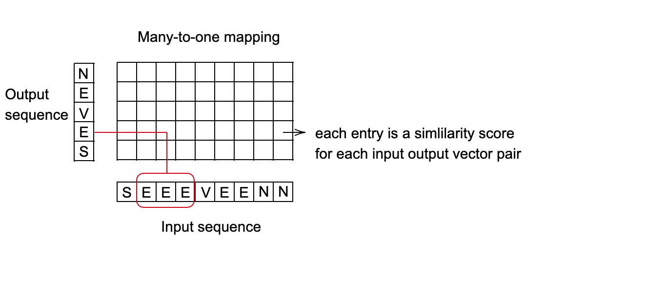
Fig. 3: Many-to-one mapping setup

Energy-Based Models (Part IV) - Loss Function

Architecture and Loss Functional

Family of energy functions: $\mathcal{E} = {E(W,Y, X) : W \in \mathcal{W}}$.

Training set: $S = {(X^i, Y^i): i = 1 \cdots P}$

Loss functional: $\mathcal{L} (E, S)$

• Functional means a function of another function. In our case, the functional $\mathcal{L} (E, S)$ is a function of the energy function $E$.
• Because $E$ is parametrised by $W$, we can turn the functional to a loss function of $W$: $\mathcal{L} (W, S)$
• Measures the quality of an energy function on training set
• Invariant under permutations and repetitions of the samples.

Training: $W^* = \arg\min_{W\in \mathcal{W}} \mathcal{L}(W, S)$.

Form of the loss functional:

• $L(Y^i, E(W, \mathcal{Y}, X^i))$ is per-sample loss
• $Y^i$ is desired answer, can be category or a whole image, etc.
• $E(W, \mathcal{Y}, X^i)$ is energy surface for a given $X_i$ as $Y$ varies
• $R(W)$ is regulariser

Designing a Good Loss Function

Push down on the energy of the correct answer.

Push up on the energies of the incorrect answers, particularly if they are smaller than the correct one.

Examples of Loss Functions

Energy Loss

This loss function simply pushes down on the energy of the correct answer. If the network is not designed properly, it might end up with a mostly flat energy function as you only trying to make the energy of the correct answer small but not pushing up the energy elsewhere. Thus, the system might collapses.

Negative Log-Likelihood Loss

This loss function pushes down on the energy of the correct answer while pushing up on the energies of all answers in proportion to their probabilities. This reduces to the perceptron loss when $\beta \rightarrow \infty$. It has been used for a long time in many communities for discriminative training with structured outputs.

A probabilistic model is an EBM in which:

• The energy can be integrated over Y (the variable to be predicted)
• The loss function is the negative log-likelihood

Perceptron Loss

Very similar to the perceptron loss from 60+ years ago, and it’s always positive because the minimum is also taken over $Y^i$, so $E(W,Y^i,X^i)-\min_{Y\in\mathcal Y} E(W,Y,X^i)\geq E(W,Y^i,X^i)-E(W,Y^i,X^i)=0$. The same computation shows that it give exactly zero only when $Y^i$ is the correct answer.

This loss makes the energy of the correct answer small, and at the same time, makes the energy for all other answers as large as possible. However, this loss does not prevent the function from giving the same value to every incorrect answer $Y^i$, so in this sense, it is a bad loss function for non-linear systems. To improve this loss, we define the most offending incorrect answer.

Generalized Margin Loss

Most offending incorrect answer: discrete case Let $Y$ be a discrete variable. Then for a training sample $(X^i,Y^i)$, the most offending incorrect answer $\bar Y^i$ is the answer that has the lowest energy among all possible answers that are incorrect:

Most offending incorrect answer: continuous case Let $Y$ be a continuous variable. Then for a training sample $(X^i,Y^i)$, the most offending incorrect answer $\bar Y^i$ is the answer that has the lowest energy among all answers that are at least $\epsilon$ away from the correct answer:

In the discrete case, the most offending incorrect answer is the one with smallest energy that isn’t the correct answer. In the continuous case, the energy for $Y$ extremely close to $Y^i$ should be close to $E(W,Y^i,X^i)$. Furthermore, the $\text{argmin}$ evaluated over $Y$ not equal to $Y^i$ would be 0. As a result, we pick a distance $\epsilon$ and decide that only $Y$’s at least $\epsilon$ from $Y_i$ should be considered the “incorrect answer”. This is why the optimization is only over $Y$’s of distance at least $\epsilon$ from $Y^i$.

If the energy function is able to ensure that the energy of the most offending incorrect answer is higher than the energy of the correct answer by some margin, then this energy function should work well.

Examples of Generalized Margin Loss Functions

Hinge Loss

Where $\bar Y^i$ is the most offending incorrect answer. This loss enforces that the difference between the correct answer and the most offending incorrect answer be at least $m$.

Fig. 4: Hinge Loss

Q: How do you pick $m$?

A: It’s arbitrary, but it affects the weights of the last layer.

Log Loss

This can be thought of as a “soft” hinge loss. Instead of composing the difference of the correct answer and the most offending incorrect answer with a hinge, it’s now composed with a soft hinge. This loss tries to enforce an “infinite margin”, but because of the exponential decay of the slope it doesn’t happen.

Fig. 5: Log Loss

Square-Square Loss

This loss combines the square of the energy with a square hinge. The combination tries to minimize the energy and but enforce margin at least $m$ on the most offending incorrect answer. This is very similar to the loss used in Siamese nets.

Other Losses

There are a whole bunch. Here is a summary of good and bad loss functions.

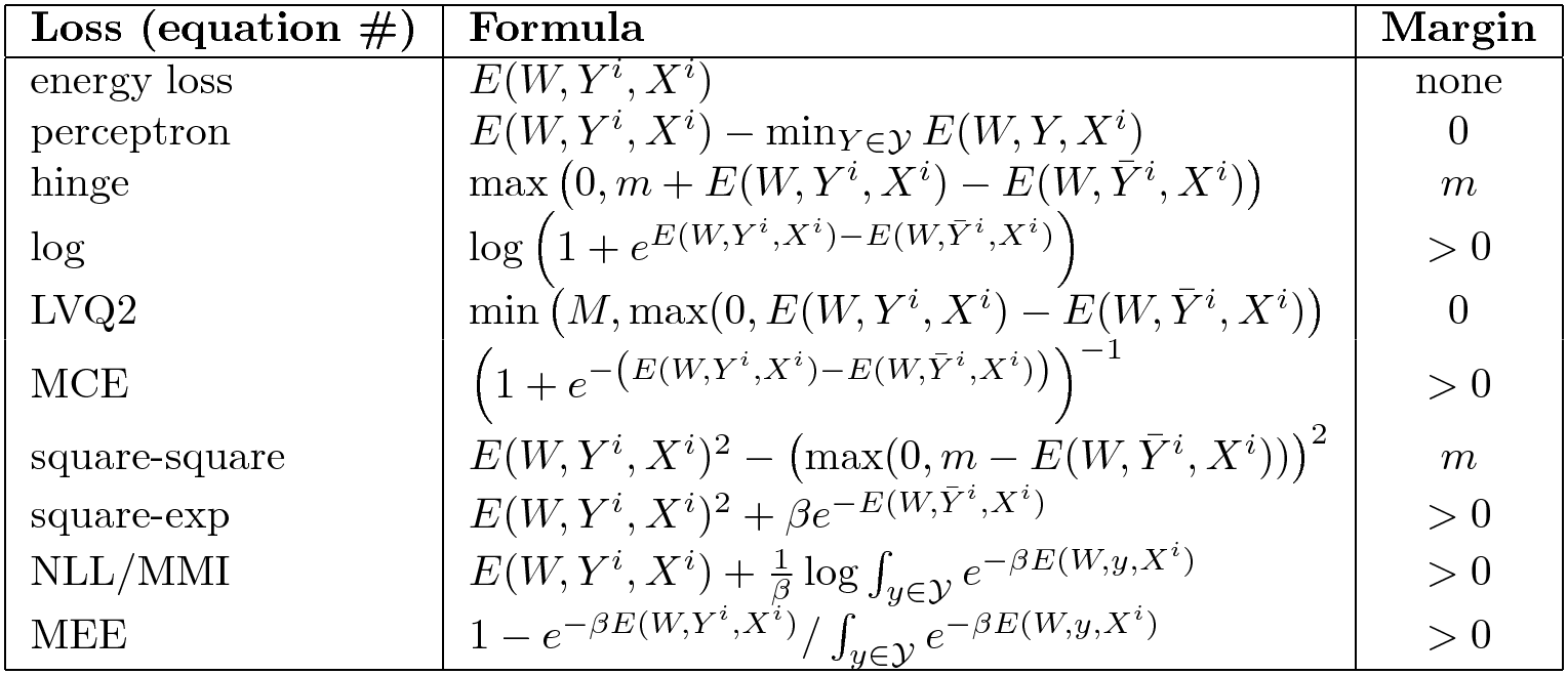
Fig. 6: Selection of EBM loss functions

The right-hand column indicates if the energy function enforces a margin. The plain old energy loss does not push up anywhere, so it doesn’t have a margin. The energy loss doesn’t work for every problem. The perceptron loss works if you have a linear parametrisation of your energy but not in general. Some of them have a finite margin like the hinge loss, and some have an infinite margin like the soft hinge.

Q: How is the most offending incorrect answer found $\bar Y_i$ found in the continuous case?

A: You want to push up on a point that is sufficiently far from $Y^i$, because if it’s too close, the parameters may not move much since the function defined by a neural net is “stiff”. But in general, this is hard and this is the problem that methods selecting contrastive samples try to solve. There’s no single correct way to do it.

A slightly more general form for hinge type contrastive losses is:

We assume that $Y$ is discrete, but if it were continuous, the sum would be replaced by an integral. Here, $E(W, Y^i,X^i)-E(W,y,X^i)$ is the difference of $E$ evaluated at the correct answer and some other answer. $C(Y^i,y)$ is the margin, and is generally a distance measure between $Y^i$ and $y$. The motivation is that the amount we want to push up on a incorrect sample $y$ should depend on the distance between $y$ and the correct sample $Y_i$. This can be a more difficult loss to optimize.