Discriminative Recurrent Sparse Auto-Encoder and Group Sparsity

Discriminative recurrent sparse autoencoder (DrSAE)

The idea of DrSAE consists of combining sparse coding, or the sparse auto-encoder, with discriminative training.

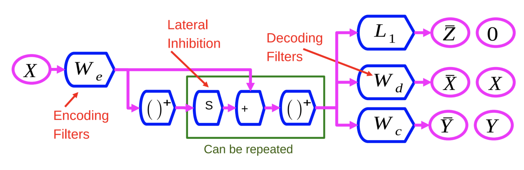
Fig 1: Discriminative Recurrent Sparse Auto-Encoder Network

The encoder, $W_e$, is similar to the encoder in the LISTA method. The $X$ variable is run through $W_e$, and then through a non-linearity. This result is then multiplied by another learned matrix, $S$, and added to $W_e$. Then it is sent through another non-linearity. This process can be repeated a number of times, with each repetition as a layer.

We train this neural network with 3 different criteria:

1. $L_1$: Apply $L_1$ criterion on the feature vector $Z$ to make it sparse.
2. Reconstruct $X$: This is done using a decoding matrix that reproduces the input on the output. This is done by minimizing square error, indicated by $W_d$ in Figure 1.
3. Add a Third Term: This third term, indicated by $W_c$, is a simple linear classifier which attempts to predict a category.

The system is trained to minimize all 3 of these criteria at the same time.

The advantage of this is by forcing the system to find representations that can reconstruct the input, then you’re basically biasing the system towards extracting features that contain as much information about the input as possible. In other words, it enriches the features.

Group Sparsity

The idea here is to generate sparse features, but not just normal features that are extracted by convolutions, but to basically produce features that are sparse after pooling.

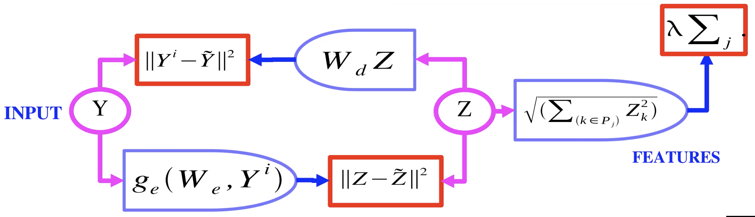
Fig 2: Auto-Encoder with Group Sparsity

Figure 2 shows an example of an auto-encoder with group sparsity. Here, instead of the latent variable $Z$ going to an $L_1$, it goes through basically an $L_2$ over groups. So you take the $L_2$ norm for each component in a group of $Z$, and take the sum of those norms. So now that is what is used as the regulariser, so we can have sparsity on groups of $Z$. These groups, or pools of features, tend to group together features that are similar to one another.

AE with group sparsity: questions and clarification

Q: Can a similar strategy used in the first slide with classifier and regulariser be applied for VAE?

A: Adding noise and forcing sparsity in a VAE are two ways of reducing the information that the latent variable/code. Prevent learning of an identity function.

Q: In slide “AE with Group Sparsity”, what is $P_j$?

A: $p$ is a pool of features. For a vector $z$, it would be a subset of the values in $z$.

Q: Clarification on feature pooling.

A: (Yann draws representation of AE with group sparsity) Encoder produces latent variable $z$, which is regularized using the $L_2$ norm of pooled features. This $z$ is used by the decoder for image reconstruction.

Q: Does group regularization help with grouping similar features?

A: The answer is unclear, work done here was done before computational power/ data was readily available. Techniques have not been brought back to the forefront.

Image level training, local filters but no weight sharing

The answer about whether it helps is not clear. People interested in this are either interested in image restoration or some kind of self-supervised learning. This would work well when dataset was very small. When you have an encoder and decoder that is convolutional and you train with group sparsity on complex cells, after you are done pre-training, the system you get rid of the decoder and only use the encoder as a feature extractor, say the first layer of the convolutional net and you stick a second layer on top of it.

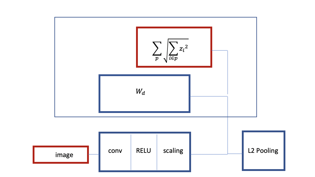
Fig 3: Structure of Convolutional RELU with Group Sparsity

As can be seen above, you start with an image, you have an encoder which is basically Convolution RELU and some kind of scaling layer after this. You train with group sparsity. You have a linear decoder and a criterion which is group by 1. You take the group sparsity as a regulariser. This is like L2 pooling with an architecture similar to group sparsity.

You can also train another instance of this network. This time, you can add more layers and have a decoder with the L2 pooling and sparsity criterion, train it to reconstruct its input with pooling on top. This will create a pretrained 2-layer convolutional net. This procedure is also called Stacked Autoencoder. The main characteristic here is that it is trained to produce invariant features with group sparsity.

Q : Should we use all possible sub-trees as groups?

A : It’s up to you, you can use multiple trees if you want. We can train the tree with a bigger tree than necessary and then removes branches rarely used.

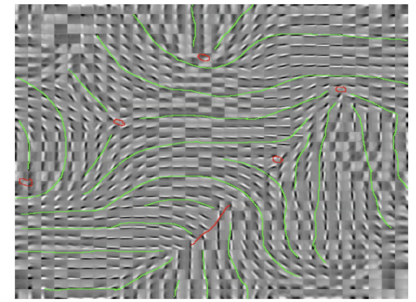
Fig 4: Image Level Training, local filters but no weight sharing

These are called pin-wheel patterns. This is a kind of organisation of the features. The orientation varies continuously as you go around those red dots. If we take one of those red dots and if do a little circle around the red dots, you notice that the orientation of the extractor kind of varies continuously as you move around. Similar trends are observed in the brain.

Q : Is the group sparsity term trained to have a small value?

It is a regulariser. The term itself is not trained, it’s fixed. It’s just the L2 norm of the groups and the groups are predetermined. But, because it is a criterion, it determines what the encoder and decoder will do and what sort of features will be extracted.

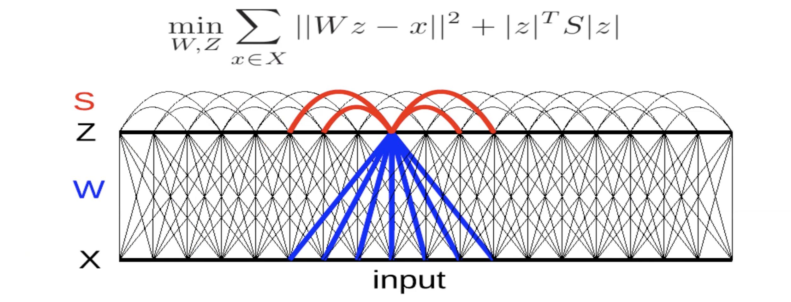
Fig 5: Invariant Features through Lateral Inhibition

Here, there is a linear decoder with square reconstruction error. There is a criterion in the energy. The matrix $S$ is either determined by hand or learned so as to maximise this term. If the terms in $S$ are positive and large, it implies that the system does not want $z_i$ and $z_j$ to be on at the same time. Thus, it is sort of a mutual inhibition (called lateral inhibition in neuroscience). Thus, you try to find a value for $S$ that is as large as possible.

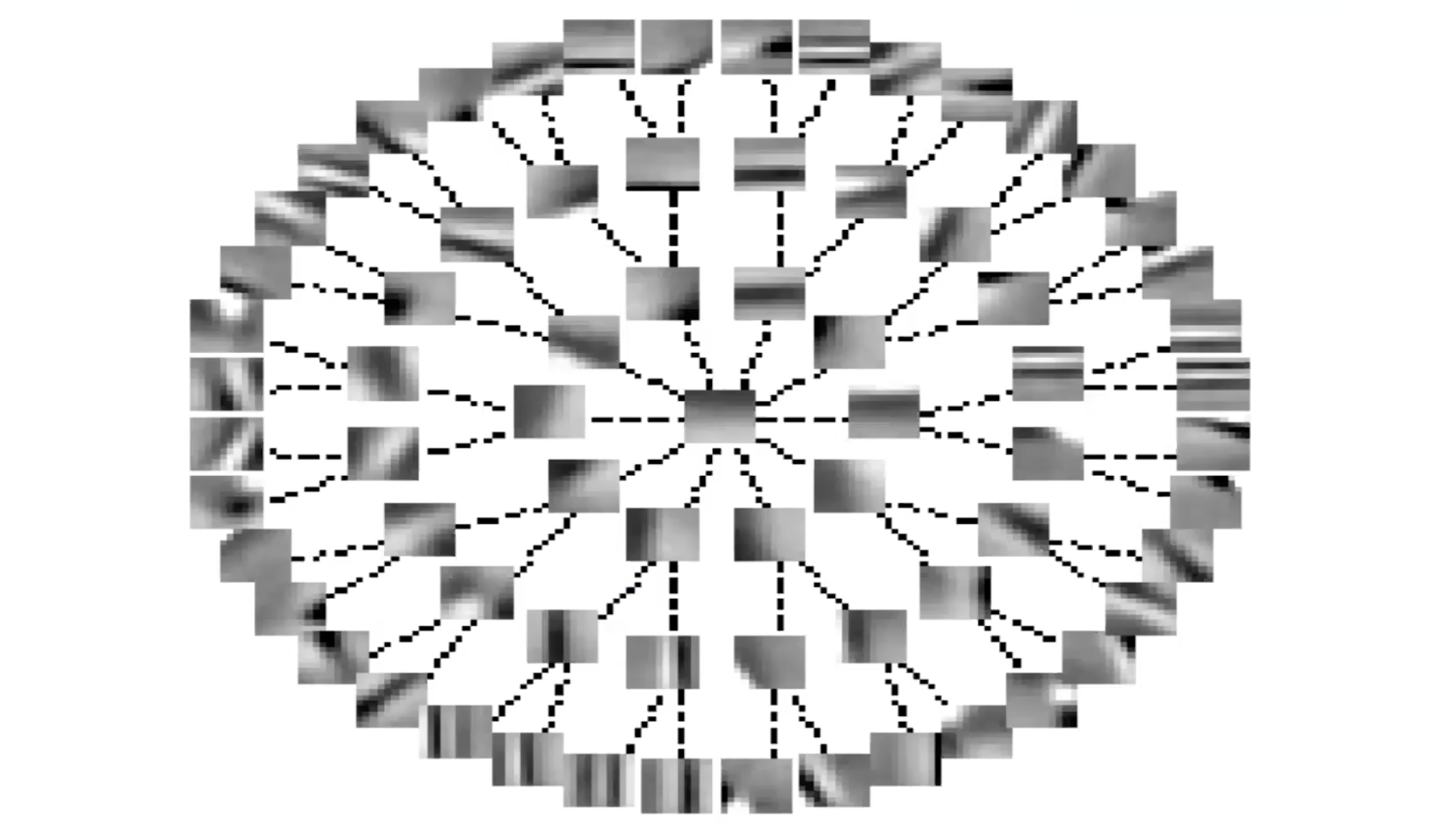
Fig 6: Invariant Features through Lateral Inhibition (Tree Form)

If you organise S in terms of a tree, the lines represent the zero terms in the $S$ matrix. Whenever you don’t have a line, there is a non-zero term. So, every feature inhibits all other features except those which are up the tree or down the tree from it. This is something like the converse of group sparsity.

You see again that systems are organising features in more or less a continuous fashion. Features along the branch of a tree represent the same feature with different levels of selectivity. Features along the periphery vary more or less continuously because there is no inhibition.

To train this system, at each iteration, you give an $x$ and find the $z$ which minimizes this energy function.Then do one step of gradient descent to update $W$. You can also do one step of gradient ascent to make the terms in $S$ larger.