ConvNet Evolutions, Architectures, Implementation Details and Advantages.

Proto-CNNs and evolution to modern CNNs

Proto-convolutional neural nets on small data sets

Inspired by Fukushima’s work on visual cortex modelling, using the simple/complex cell hierarchy combined with supervised training and backpropagation lead to the development of the first CNN at University of Toronto in ‘88-‘89 by Prof. Yann LeCun. The experiments used a small dataset of 320 ‘mouser-written’ digits. Performances of the following architectures were compared:

1. Single FC(fully connected) Layer
2. Two FC Layers
3. Locally Connected Layers w/o shared weights
4. Constrained network w/ shared weights and local connections
5. Constrained network w/ shared weights and local connections 2 (more feature maps)

The most successful networks (constrained network with shared weights) had the strongest generalizability, and form the basis for modern CNNs. Meanwhile, singler FC layer tends to overfit.

First “real” ConvNets at Bell Labs

After moving to Bell Labs, LeCunn’s research shifted to using handwritten zipcodes from the US Postal service to train a larger CNN:

• 256 (16$\times$16) input layer
• 12 5$\times$5 kernels with stride 2 (stepped 2 pixels): next layer has lower resolution
• NO separate pooling

Convolutional network architecture with pooling

The next year, some changes were made: separate pooling was introduced. Separate pooling is done by averaging input values, adding a bias, and passing to a nonlinear function (hyperbolic tangent function). The 2$\times$2 pooling was performed with a stride of 2, hence reducing resolutions by half.

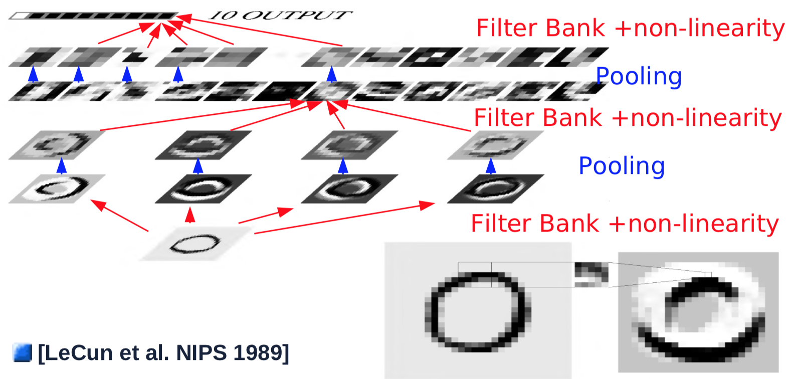
Fig. 1 ConvNet Architecture

An example of a single convolutional layer would be as follows:

1. Take an input with size 32$\times$32
2. The convolution layer passes a 5$\times$5 kernel with stride 1 over the image, resulting feature map size 28$\times$28
3. Pass the feature map to a nonlinear function: size 28$\times$28
4. Pass to the pooling layer that averages over a 2$\times$2 window with stride 2: size 14$\times$14
5. Repeat 1-4 for 4 kernels

The first-layer, simple convolution/pool combinations usually detect simple features, such as oriented edge detections. After the first convolution/pool layer, the objective is to detect combinations of features from previous layers. To do this, steps 2 to 4 are repeated with multiple kernels over previous-layer feature maps, and are summed in a new feature map:

1. A new 5$\times$5 kernel is slid over all feature maps from previous layers, with results summed up. (Note: In Prof. LeCun’s experiment in 1989 the connection is not full for computation purpose. Modern settings usually enforce full connections): size 10$\times$10
2. Pass the output of the convolution to a nonlinear function: size 10$\times$10
3. Repeat 1/2 for 16 kernels.
4. Pass the result to the pooling layer that averages over 2$\times$2 window with stride 2: size 5$\times$5 each feature map

To generate an output, the last layer of convolution is conducted, which seems like a full connections but indeed is convolutional.

1. The final convolution layer slides a 5$\times$5 kernel over all feature maps, with results summed up: size 1$\times$1
2. Pass through nonlinear function: size 1$\times$1
3. Generate the single output for one category.
4. Repeat all pervious steps for each of the 10 categories(in parallel)

See this animation on Andrej Karpathy’s website on how convolutions change the shape of the next layer’s feature maps. Full paper can be found here.

Shift equivariance

Fig. 2 Shift Equivariance

As demonstrated by the animation on the slides(here’s another example), translating the input image results in same translation of the feature maps. However, the changes in feature maps are scaled by convolution/pooling operations. E.g. the 2$\times$2 pooling with stride 2 will reduce the 1-pixel shift in input layer to 0.5-pixel shift in the following feature maps. Spatial resolution is then exchanged for increased number of feature types, i.e. making the representation more abstract and less sensitive to shifts and distortions.

Overall architecture breakdown

Generic CNN architecture can be broken down into several basic layer archetypes:

• Normalisation
  • Adjusting whitening (optional)
  • Subtractive methods e.g. average removal, high pass filtering
  • Divisive: local contrast normalisation, variance normalisation
• Filter Banks
  • Increase dimensionality
  • Projection on overcomplete basis
  • Edge detections
• Non-linearities
  • Sparsification
  • Typically Rectified Linear Unit (ReLU): $\text{ReLU}(x) = \max(x, 0)$
• Pooling
  • Aggregating over a feature map

  • Max Pooling: $\text{MAX}= \text{Max}_i(X_i)$

  • LP-Norm Pooling: \(\text{L}p= \left(\sum_{i=1}^n \|X_i\|^p \right)^{\frac{1}{p}}\)

  • Log-Prob Pooling: $\text{Prob}= \frac{1}{b} \left(\sum_{i=1}^n e^{b X_i} \right)$

LeNet5 and digit recognition

Implementation of LeNet5 in PyTorch

LeNet5 consists of the following layers (1 being the top-most layer):

1. Log-softmax
2. Fully connected layer of dimensions 500$\times$10
3. ReLu
4. Fully connected layer of dimensions (4$\times$4$\times$50)$\times$500
5. Max Pooling of dimensions 2$\times$2, stride of 2.
6. ReLu
7. Convolution with 20 output channels, 5$\times$5 kernel, stride of 1.
8. Max Pooling of dimensions 2$\times$2, stride of 2.
9. ReLu
10. Convolution with 20 output channels, 5$\times$5 kernel, stride of 1.

The input is a 32$\times$32 grey scale image (1 input channel).

LeNet5 can be implemented in PyTorch with the following code:

class LeNet5(nn.Module):
    def __init__(self):
        super().__init__()
        self.conv1 = nn.Conv2d(1, 20, 5, 1)
        self.conv2 = nn.Conv2d(20, 20, 5, 1)
        self.fc1 = nn.Linear(4*4*50, 500)
        self.fc2 = nn.Linear(500, 10)

    def forward(self, x):
        x = F.relu(self.conv1(x))
        x = F.max_pool2d(x, 2, 2)
        x = F.relu(self.conv2(x))
        x = F.max_pool2d(x, 2, 2)
        x = x.view(-1, 4*4*50)
        x = F.relu(self.fc1)
        x = self.fc2(x)
    return F.logsoftmax(x, dim=1)

Although fc1 and fc2 are fully connected layers, they can be thought of as convolutional layers whose kernels cover the entire input. Fully connected layers are used for efficiency purposes.

The same code can be expressed using nn.Sequential, but it is outdated.

Advantages of CNN

In a fully convolutional network, there is no need to specify the size of the input. However, changing the size of the input changes the size of the output.

Consider a cursive hand-writing recognition system. We do not have to break the input image into segments. We can apply the CNN over the entire image: the kernels will cover all locations in the entire image and record the same output regardless of where the pattern is located. Applying the CNN over an entire image is much cheaper than applying it at multiple locations separately. No prior segmentation is required, which is a relief because the task of segmenting an image is similar to recognizing an image.

Example: MNIST

LeNet5 is trained on MNIST images of size 32$\times$32 to classify individual digits in the centre of the image. Data augmentation was applied by shifting the digit around, changing the size of the digit, inserting digits to the side. It was also trained with an 11-th category which represented none of the above. Images labelled by this category were generated either by producing blank images, or placing digits at the side but not the centre.

Fig. 3 Sliding Window ConvNet

The above image demonstrates that a LeNet5 network trained on 32$\times$32 can be applied on a 32$\times$64 input image to recognise the digit at multiple locations.

Feature binding problem

What is the feature binding problem?

Visual neural scientists and computer vision people have the problem of defining the object as an object. An object is a collection of features, but how to bind all of the features to form this object?

How to solve it?

We can solve this feature binding problem by using a very simple CNN: only two layers of convolutions with poolings plus another two fully connected layers without any specific mechanism for it, given that we have enough non-linearities and data to train our CNN.

Fig. 4 ConvNet Addressing Feature Binding

The above animation showcases the ability of CNN to recognize different digits by moving a single stroke around, demonstrating its ability to address feature binding problems, i.e. recognizing features in a hierarchical, compositional way.

Example: dynamic input length

We can build a CNN with 2 convolution layers with stride 1 and 2 pooling layers with stride 2 such that the overall stride is 4. Thus, if we want to get a new output, we need to shift our input window by 4. To be more explicit, we can see the figure below (green units). First, we have an input of size 10, and we perform convolution of size 3 to get 8 units. After that, we perform pooling of size 2 to get 4 units. Similarly, we repeat the convolution and pooling again and eventually we get 1 output.

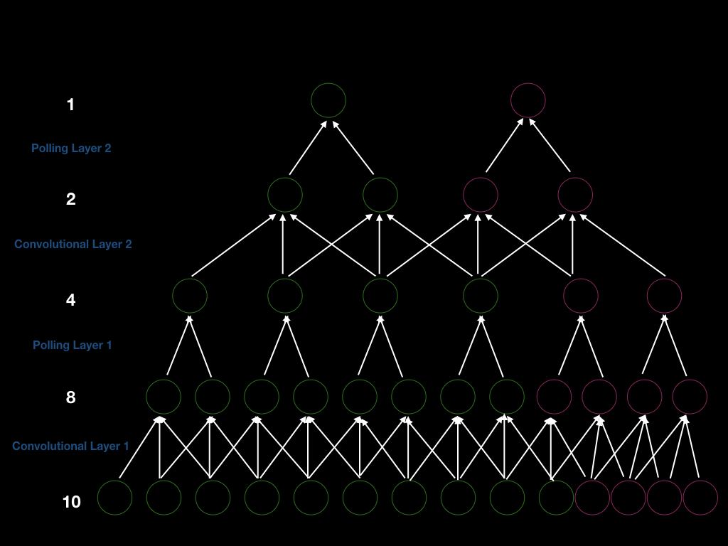
Fig. 5 ConvNet Architecture On Variant Input Size Binding

Let’s assume we add 4 units at the input layer (pink units above), so that we can get 4 more units after the first convolution layer, 2 more units after the first pooling layer, 2 more units after the second convolution layer, and 1 more output. Therefore, window size to generate a new output is 4 (2 stride $\times$2). Moreover, this is a demonstration of the fact that if we increase the size of the input, we will increase the size of every layer, proving CNNs’ capability in handling dynamic length inputs.

What are CNN good for

CNNs are good for natural signals that come in the form of multidimensional arrays and have three major properties:

1. Locality: The first one is that there is a strong local correlation between values. If we take two nearby pixels of a natural image, those pixels are very likely to have the same colour. As two pixels become further apart, the similarity between them will decrease. The local correlations can help us detect local features, which is what the CNNs are doing. If we feed the CNN with permuted pixels, it will not perform well at recognizing the input images, while FC will not be affected. The local correlation justifies local connections.
2. Stationarity: Second character is that the features are essential and can appear anywhere on the image, justifying the shared weights and pooling. Moreover, statistical signals are uniformly distributed, which means we need to repeat the feature detection for every location on the input image.
3. Compositionality: Third character is that the natural images are compositional, meaning the features compose an image in a hierarhical manner. This justifies the use of multiple layers of neurons, which also corresponds closely with Hubel and Weisel’s research on simple and complex cells.

Furthermore, people make good use of CNNs on videos, images, texts, and speech recognition.