Visualization of neural networks parameter transformation and fundamental concepts of convolution

Visualization of neural networks

In this section we will visualise the inner workings of a neural network.

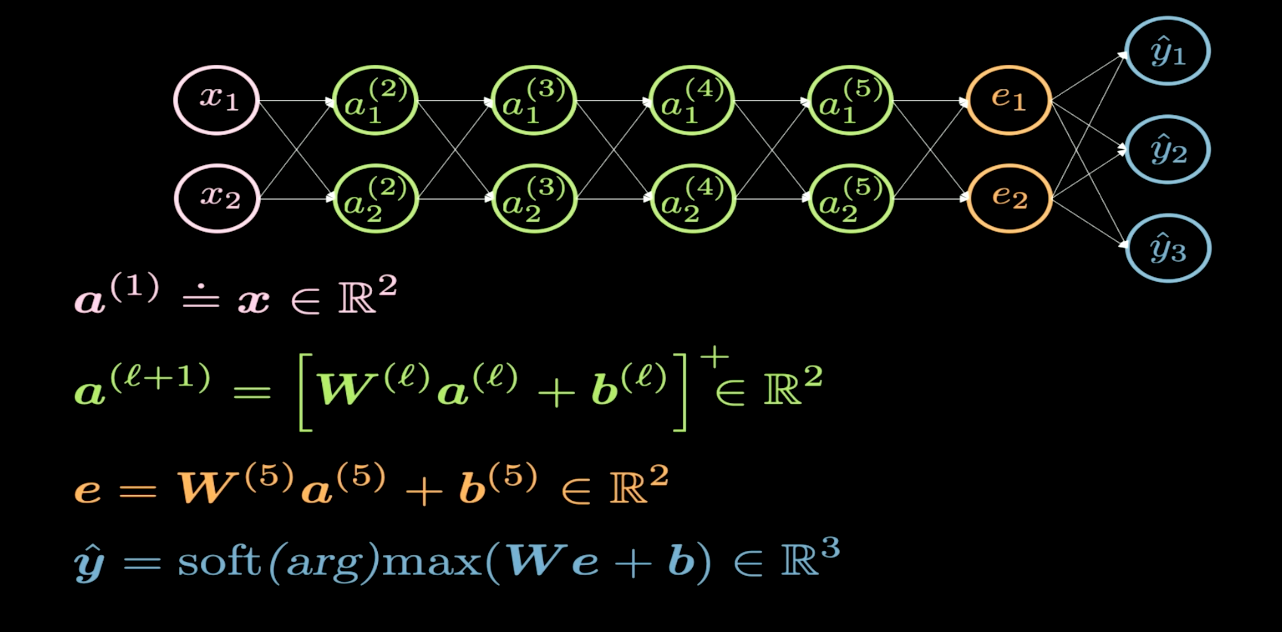
Fig. 1 Network Structure

Figure 1 depicts the structure of the neural network we would like to visualise. Typically, when we draw the structure of a neural network, the input appears on the bottom or on the left, and the output appears on the top side or on the right. In Figure 1, the pink neurons represent the inputs, and the blue neurons represent the outputs. In this network, we have 4 hidden layers (in green), which means we have 6 layers in total (4 hidden layers + 1 input layer + 1 output layer). In this case, we have 2 neurons per hidden layer, and hence the dimension of the weight matrix ($W$) for each layer is 2-by-2. This is because we want to transform our input plane into another plane that we can visualize.

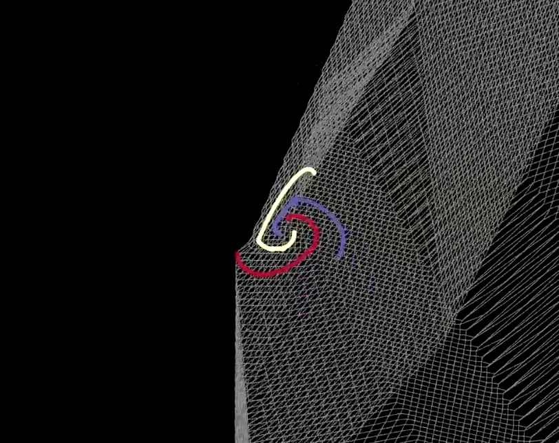
Fig. 2 Visualization of folding space

The transformation of each layer is like folding our plane in some specific regions as shown in Figure 2. This folding is very abrupt, this is because all the transformations are performed in the 2D layer. In the experiment, we find that if we have only 2 neurons in each hidden layer, the optimization will take longer; the optimization is easier if we have more neurons in the hidden layers. This leaves us with an important question to consider: Why is it harder to train the network with fewer neurons in the hidden layers? You should consider this question yourself and we will return to it after the visualization of $\texttt{ReLU}$.

(a)	(b)

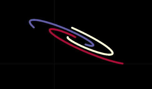
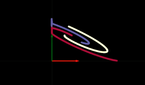
When we step through the network one hidden layer at a time, we see that with each layer we perform some affine transformation followed by applying the non-linear ReLU operation, which eliminates any negative values. In Figures 3(a) and (b), we can see the visualisation of ReLU operator. The ReLU operator helps us to do non-linear transformations. After mutliple steps of performing an affine transformation followed by the ReLU operator, we are eventually able to linearly separate the data as can be seen in Figure 4.

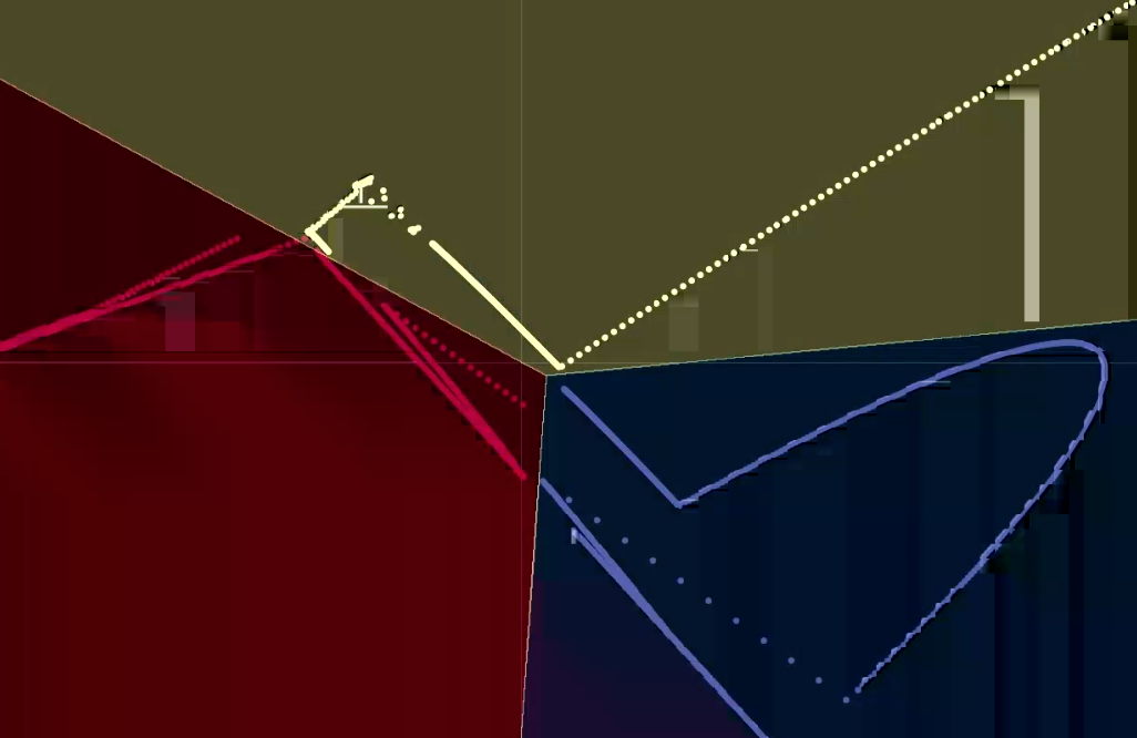
Fig. 4 Visualization of Outputs

This provides us with some insight into why the 2-neuron hidden layers are harder to train. Our 6-layer network has one bias in each hidden layers. Therefore if one of these biases moves points out of top-right quadrant, then applying the ReLU operator will eliminate these points to zero. After that, no matter how later layers transform the data, the values will remain zero. We can make a neural network easier to train by making the network “fatter” - i.e. adding more neurons in hidden layers - or we can add more hidden layers, or a combination of the two methods. Throughout this course we will explore how to determine the best network architecture for a given problem, stay tuned.

Parameter transformations

General parameter transformation means that our parameter vector $w$ is the output of a function. By this transformation, we can map original parameter space into another space. In Figure 5, $w$ is actually the output of $H$ with the parameter $u$. $G(x,w)$ is a network and $C(y,\bar y)$ is a cost function. The backpropagation formula is also adapted as follows,

These formulas are applied in a matrix form. Note that the dimensions of the terms should be consistent. The dimension of $u$,$w$,$\frac{\partial H}{\partial u}^\top$,$\frac{\partial C}{\partial w}^\top$ are $[N_u \times 1]$,$[N_w \times 1]$,$[N_u \times N_w]$,$[N_w \times 1]$, respectively. Therefore, the dimension of our backpropagation formula is consistent.

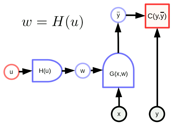
Fig. 5 General Form of Parameter Transformations

A simple parameter transformation: weight sharing

A Weight Sharing Transformation means $H(u)$ just replicates one component of $u$ into multiple components of $w$. $H(u)$ is like a Y branch to copy $u_1$ to $w_1$, $w_2$. This can be expressed as,

We force shared parameters to be equal, so the gradient w.r.t. to shared parameters will be summed in the backprop. For example the gradient of the cost function $C(y, \bar y)$ with respect to $u_1$ will be the sum of the gradient of the cost function $C(y, \bar y)$ with respect to $w_1$ and the gradient of the cost function $C(y, \bar y)$ with respect to $w_2$.

Hypernetwork

A hypernetwork is a network where the weights of one network is the output of another network. Figure 6 shows the computation graph of a “hypernetwork”. Here the function $H$ is a network with parameter vector $u$ and input $x$. As a result, the weights of $G(x,w)$ are dynamically configured by the network $H(x,u)$. Although this is an old idea, it remains very powerful.

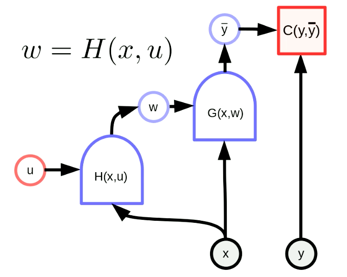
Fig. 6 "Hypernetwork"

Motif detection in sequential data

Weight sharing transformation can be applied to motif detection. Motif detection means to find some motifs in sequential data like keywords in speech or text. One way to achieve this, as shown in Figure 7, is to use a sliding window on data, which moves the weight-sharing function to detect a particular motif (i.e. a particular sound in speech signal), and the outputs (i.e. a score) goes into a maximum function.

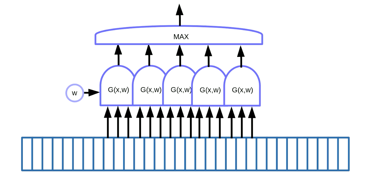
Fig. 7 Motif Detection for Sequential Data

In this example we have 5 of those functions. As a result of this solution, we sum up five gradients and backpropagate the error to update the parameter $w$. When implementing this in PyTorch, we want to prevent the implicit accumulation of these gradients, so we need to use zero_grad() to initialize the gradient.

Motif detection in images

The other useful application is motif detection in images. We usually swipe our “templates” over images to detect the shapes independent of position and distortion of the shapes. A simple example is to distinguish between “C” and “D”, as Figure 8 shows. The difference between “C” and “D” is that “C” has two endpoints and “D” has two corners. So we can design “endpoint templates” and “corner templates”. If the shape is similar to the “templates”, it will have thresholded outputs. Then we can distinguish letters from these outputs by summing them up. In Figure 8, the network detects two endpoints and zero corners, so it activates “C”.

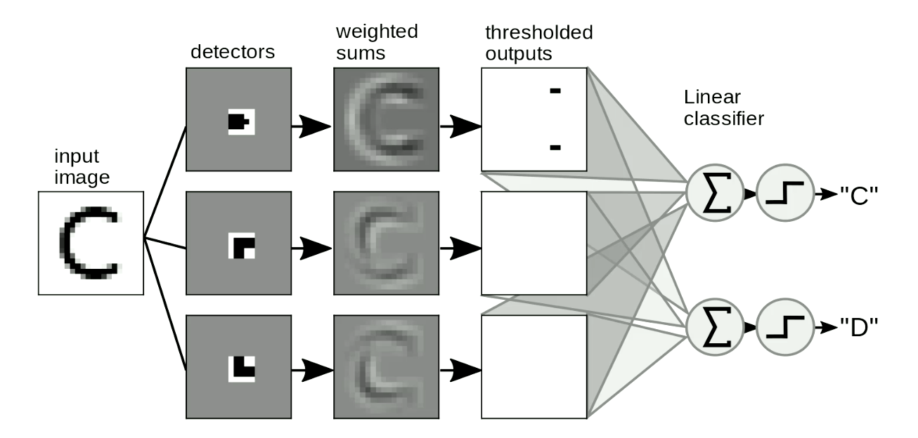
Fig. 8 Motif Detection for Images

It is also important that our “template matching” should be shift-invariant - when we shift the input, the output (i.e. the letter detected) shouldn’t change. This can be solved with weight sharing transformation. As Figure 9 shows, when we change the location of “D”, we can still detect the corner motifs even though they are shifted. When we sum up the motifs, it will activate the “D” detection.

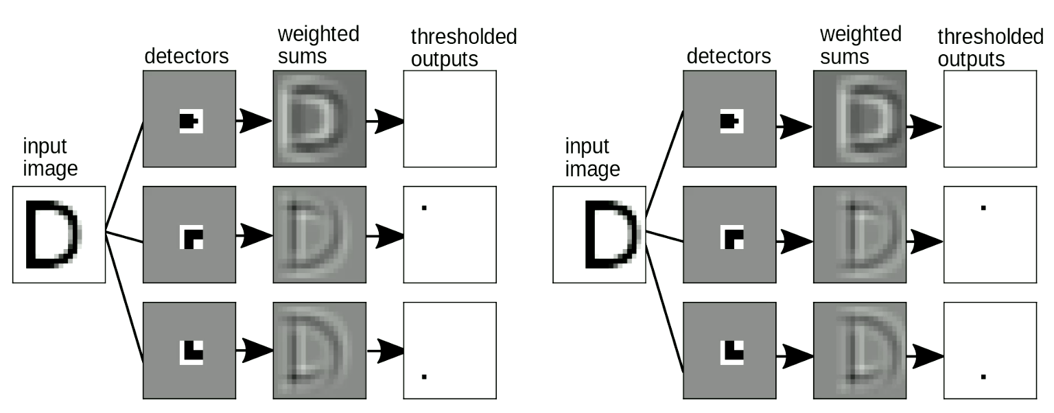
Fig. 9 Shift Invariance

This hand-crafted method of using local detectors and summation to for digit-recognition was used for many years. But it presents us with the following problem: How can we design these “templates” automatically? Can we use neural networks to learn these “templates”? Next, We will introduce the concept of convolutions , that is, the operation we use to match images with “templates”.

Discrete convolution

Convolution

The precise mathematical definition of a convolution in the 1-dimensional case between input $x$ and $w$ is:

In words, the $i$-th output is computed as the dot product between the reversed $w$ and a window of the same size in $x$. To compute the full output, start the window at the beginning, shift this window by one entry each time and repeat until $x$ is exhausted.

Cross-correlation

In practice, the convention adopted in deep learning frameworks such as PyTorch is slightly different. Convolution in PyTorch is implemented where $w$ is not reversed:

Mathematicians call this formulation “cross-correlation”. In our context, this difference is just a difference in convention. Practically, cross-correlation and convolution can be interchangeable if one reads the weights stored in memory forward or backward.

Being aware of this difference is important, for example, when one want to make use of certain mathematical properties of convolution/correlation from mathematical texts.

Higher dimensional convolution

For two dimensional inputs such as images, we make use of the two dimensional version of convolution:

This definition can easily be extended beyond two dimensions to three or four dimensions. Here $w$ is called the convolution kernel

Regular twists that can be made with the convolutional operator in DCNNs

1. Striding: instead of shifting the window in $x$ one entry at a time, one can do so with a larger step (for example two or three entries at a time). Example: Suppose the input $x$ is one dimensional and has size of 100 and $w$ has size 5. The output size with a stride of 1 or 2 is shown in the table below:

1. Padding: Very often in designing Deep Neural Networks architectures, we want the output of convolution to be of the same size as the input. This can be achieved by padding the input ends with a number of (typically) zero entries, usually on both sides. Padding is done mostly for convenience. It can sometimes impact performance and result in strange border effects, that said, when using a ReLU non-linearity, zero padding is not unreasonable.

Deep Convolution Neural Networks (DCNNs)

As previously described, deep neural networks are typically organized as repeated alternation between linear operators and point-wise nonlinearity layers. In convolutional neural networks, the linear operator will be the convolution operator described above. There is also an optional third type of layer called the pooling layer.

The reason for stacking multiple such layers is that we want to build a hierarchical representation of the data. CNNs do not have to be limited to processing images, they have also been successfully applied to speech and language. Technically they can be applied to any type of data that comes in the form of arrays, although we also these arrays to satisfy certain properties.

Why would we want to capture the hierarchical representation of the world? Because the world we live in is compositional. This point is alluded to in previous sections. Such hierarchical nature can be observed from the fact that local pixels assemble to form simple motifs such as oriented edges. These edges in turn are assembled to form local features such as corners, T-junctions, etc. These edges are assembled to form motifs that are even more abstract. We can keep building on these hierarchical representation to eventually form the objects we observe in the real world.

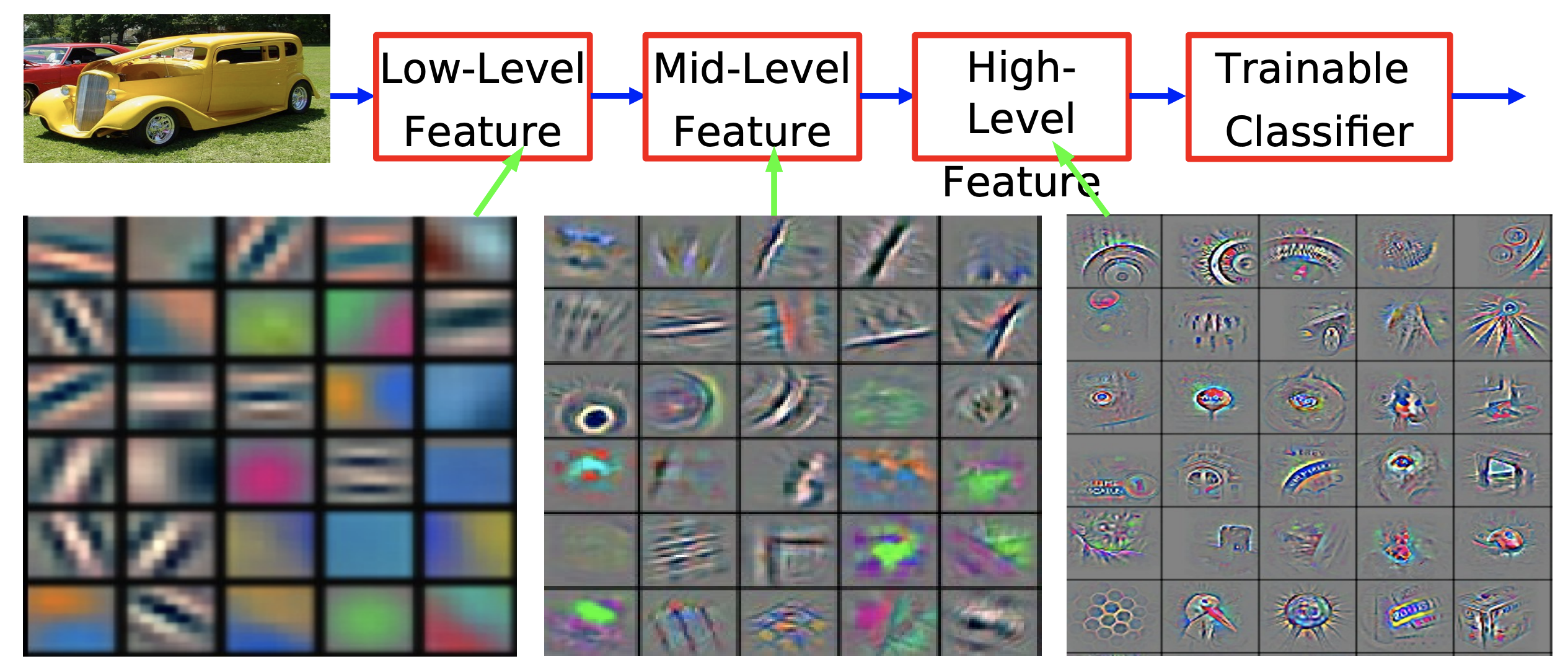
Figure 10. Feature visualization of convolutional net trained on ImageNet from [Zeiler & Fergus 2013]

This compositional, hierarchical nature we observe in the natural world is therefore not just the result of our visual perception, but also true at the physical level. At the lowest level of description, we have elementary particles, which assembled to form atoms, atoms together form molecules, we continue to build on this process to form materials, parts of objects and eventually full objects in the physical world.

The compositional nature of the world might be the answer to Einstein’s rhetorical question on how humans understand the world they live in:

The most incomprehensible thing about the universe is that it is comprehensible.

The fact that humans understand the world thanks to this compositional nature still seems like a conspiracy to Yann. It is, however, argued that without compositionality, it will take even more magic for humans to comprehend the world they live in. Quoting the great mathematician Stuart Geman:

The world is compositional or God exists.

Inspirations from Biology

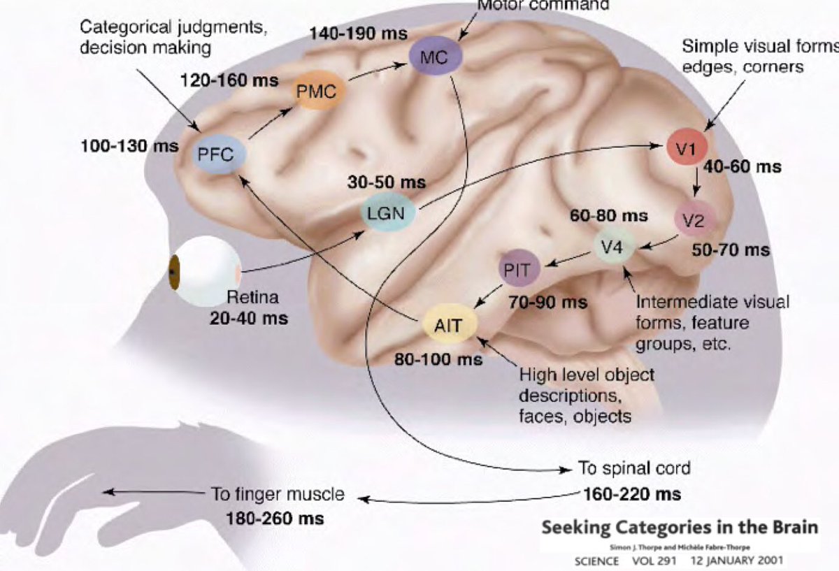
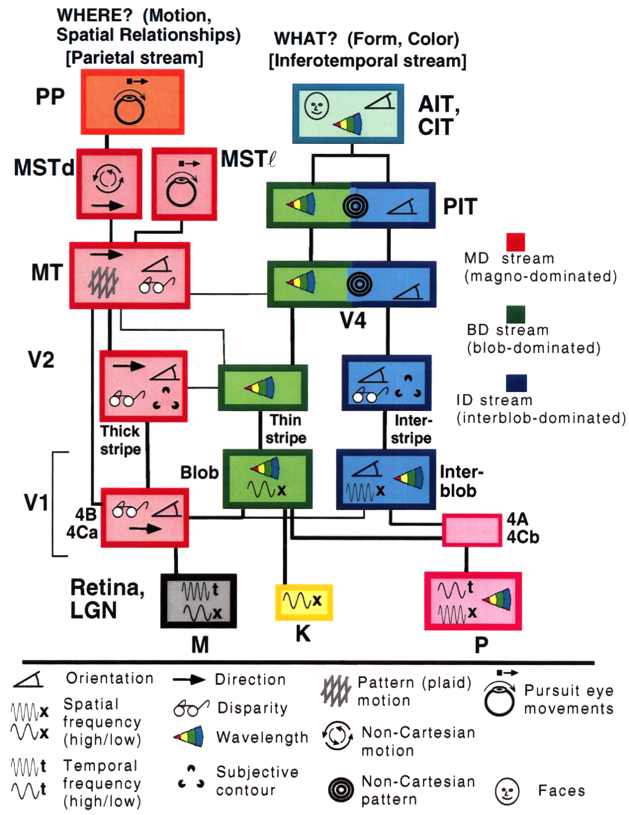
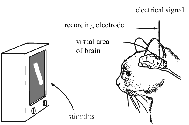
So why should Deep Learning be rooted in the idea that our world is comprehensible and has a compositional nature? Research conducted by Simon Thorpe helped motivate this further. He showed that the way we recognize everyday objects is extremely fast. His experiments involved flashing a set of images every 100ms, and then asking users to identify these images, which they were able to do successfully. This demonstrated that it takes about 100ms for humans to detect objects. Furthermore, consider the diagram below, illustrating parts of the brain annotated with the time it takes for neurons to propagate from one area to the next:

Figure 11. Simon Thorpe's model of visual information flow in the brain

Signals pass from the retina to the LGN (helps with contrast enhancement, gate control, etc.), then to the V1 primary visual cortex, V2, V4, then to the inferotemporal cortex (PIT), which is the part of the brain where categories are defined. Observations from open-brain surgery showed that if you show a human a film, neurons in the PIT will fire only when they detect certain images -- such as Jennifer Aniston or a person's grandmother -- and nothing else. The neural firings are invariant to things such as position, size, illumination, your grandmother's orientation, what she's wearing, etc. Furthermore, the fast reaction times with which humans were able to categorize these items -- barely enough time for a few spikes to get through -- demonstrates that it's possible to do this without additional time spent on complex recurrent computations. Rather, this is a single feed-forward process. These insights suggested that we could develop a neural network architecture which is completely feed-forward, yet still able to solve the problem of recognition, in a way that is invariant to irrelevant transformations of the input. One further insight from the human brain comes from Gallant & Van Essen, whose model of the human brain illustrates two distinct pathways:

Figure 12. Gallen & Van Essen's model of dorsal & ventral pathways in the brain

The right side shows the ventral pathway, which tells you what you're looking at, while the left side shows the dorsal pathway, which identifies locations, geometry, and motion. They seem fairly separate in the human (and primate) visual cortex (with a few interactions between them of course). ### Hubel & Weisel's contributions (1962)

Figure 13. Hubel & Weisel's experiments with visual stimuli in cat brains

Hubel and Weisel experiments used electrodes to measure neural firings in cat brains in response to visual stimuli. They discovered that neurons in the V1 region are only sensitive to certain areas of a visual field (called "receptive fields"), and detect oriented edges in that area. For example, they demonstrated that if you showed the cat a vertical bar and start rotating it, at a particular angle the neuron will fire. Similarly, as the bar moves away from that angle, the activation of the neuron diminishes. These activation-selective neurons Hubel & Weisel named "simple cells", for their ability to detect local features. They also discovered that if you move the bar out of the receptive field, that particular neuron doesn't fire any more, but another neuron will. There are local feature detectors corresponding to all areas of the visual field, hence the idea that the human brain processes visual information as a collection of "convolutions". Another type of neuron, which they named "complex cells", aggregate the output of multiple simple cells within a certain area. We can think of these as computing an aggregate of the activations using a function such as maximum, sum, sum of squares, or any other function not depending on the order. These complex cells detect edges and orientations in a region, regardless of where those stimuli lie specifically within the region. In other words, they are shift-invariant with respect to small variations in positions of the input. ### Fukushima's contributions (1982)

Figure 14. Fukushima's CNN model

Fukushima was the first to implement the idea of multiple layers of simple cells and complex cells with computer models, using a dataset of handwritten digits. Some of these feature detectors were hand-crafted or learned, though the learning used unsupervised clustering algorithms, trained separately for each layer, as backpropagation was not yet in use. Yann LeCun came in a few years later (1989, 1998) and implemented the same architecture, but this time trained them in a supervised setting using backpropagation. This is widely regarded as the genesis of modern convolutional neural networks. (Note: Riesenhuber at MIT in 1999 also re-discovered this architecture, though he didn't use backpropagation.)