Attention and the Transformer

Attention

We introduce the concept of attention before talking about the Transformer architecture. There are two main types of attention: self attention vs. cross attention, within those categories, we can have hard vs. soft attention.

As we will later see, transformers are made up of attention modules, which are mappings between sets, rather than sequences, which means we do not impose an ordering to our inputs/outputs.

Self Attention (I)

Consider a set of $t$ input $\boldsymbol{x}$’s:

where each $\boldsymbol{x}_i$ is an $n$-dimensional vector. Since the set has $t$ elements, each of which belongs to $\mathbb{R}^n$, we can represent the set as a matrix $\boldsymbol{X}\in\mathbb{R}^{n \times t}$.

With self-attention, the hidden representation $h$ is a linear combination of the inputs:

Using the matrix representation described above, we can write the hidden layer as the matrix product:

where $\boldsymbol{a} \in \mathbb{R}^t$ is a column vector with components $\alpha_i$.

Note that this differs from the hidden representation we have seen so far, where the inputs are multiplied by a matrix of weights.

Depending on the constraints we impose on the vector $\vect{a}$, we can achieve hard or soft attention.

Hard Attention

With hard-attention, we impose the following constraint on the alphas: $\Vert\vect{a}\Vert_0 = 1$. This means $\vect{a}$ is a one-hot vector. Therefore, all but one of the coefficients in the linear combination of the inputs equals zero, and the hidden representation reduces to the input $\boldsymbol{x}_i$ corresponding to the element $\alpha_i=1$.

Soft Attention

With soft attention, we impose that $\Vert\vect{a}\Vert_1 = 1$. The hidden representations is a linear combination of the inputs where the coefficients sum up to 1.

Self Attention (II)

Where do the $\alpha_i$ come from?

We obtain the vector $\vect{a} \in \mathbb{R}^t$ in the following way:

Where $\beta$ represents the inverse temperature parameter of the $\text{soft(arg)max}(\cdot)$. $\boldsymbol{X}^{\top}\in\mathbb{R}^{t \times n}$ is the transposed matrix representation of the set $\lbrace\boldsymbol{x}_i \rbrace_{i=1}^t$, and $\boldsymbol{x}$ represents a generic $\boldsymbol{x}_i$ from the set. Note that the $j$-th row of $X^{\top}$ corresponds to an element $\boldsymbol{x}_j\in\mathbb{R}^n$, so the $j$-th row of $\boldsymbol{X}^{\top}\boldsymbol{x}$ is the scalar product of $\boldsymbol{x}_j$ with each $\boldsymbol{x}_i$ in $\lbrace \boldsymbol{x}_i \rbrace_{i=1}^t$.

The components of the vector $\vect{a}$ are also called “scores” because the scalar product between two vectors tells us how aligned or similar two vectors are. Therefore, the elements of $\vect{a}$ provide information about the similarity of the overall set to a particular $\boldsymbol{x}_i$.

The square brackets represent an optional argument. Note that if $\arg\max(\cdot)$ is used, we get a one-hot vector of alphas, resulting in hard attention. On the other hand, $\text{soft(arg)max}(\cdot)$ leads to soft attention. In each case, the components of the resulting vector $\vect{a}$ sum to 1.

Generating $\vect{a}$ this way gives a set of them, one for each $\boldsymbol{x}_i$. Moreover, each $\vect{a}_i \in \mathbb{R}^t$ so we can stack the alphas in a matrix $\boldsymbol{A}\in \mathbb{R}^{t \times t}$.

Since each hidden state is a linear combination of the inputs $\boldsymbol{X}$ and a vector $\vect{a}$, we obtain a set of $t$ hidden states, which we can stack into a matrix $\boldsymbol{H}\in \mathbb{R}^{n \times t}$.

Key-value store

A key-value store is a paradigm designed for storing (saving), retrieving (querying) and managing associative arrays (dictionaries / hash tables).

For example, say we wanted to find a recipe to make lasagne. We have a recipe book and search for “lasagne” - this is the query. This query is checked against all possible keys in your dataset - in this case, this could be the titles of all the recipes in the book. We check how aligned the query is with each title to find the maximum matching score between the query and all the respective keys. If our output is the argmax function - we retrieve the single recipe with the highest score. Otherwise, if we use a soft argmax function, we would get a probability distribution and can retrieve in order from the most similar content to less and less relevant recipes matching the query.

Basically, the query is the question. Given one query, we check this query against every key and retrieve all matching content.

Queries, keys and values

Each of the vectors $\vect{q}, \vect{k}, \vect{v}$ can simply be viewed as rotations of the specific input $\vect{x}$. Where $\vect{q}$ is just $\vect{x}$ rotated by $\vect{W_q}$, $\vect{k}$ is just $\vect{x}$ rotated by $\vect{W_k}$ and similarly for $\vect{v}$. Note that this is the first time we are introducing “learnable” parameters. We also do not include any non-linearities since attention is completely based on orientation.

In order to compare the query against all possible keys, $\vect{q}$ and $\vect{k}$ must have the same dimensionality, i.e. $\vect{q}, \vect{k} \in \mathbb{R}^{d’}$.

However, $\vect{v}$ can be of any dimension. If we continue with our lasagne recipe example - we need the query to have the dimension as the keys, i.e. the titles of the different recipes that we’re searching through. The dimension of the corresponding recipe retrieved, $\vect{v}$, can be arbitrarily long though. So we have that $\vect{v} \in \mathbb{R}^{d’’}$.

For simplicity, here we will make the assumption that everything has dimension $d$, i.e.

So now we have a set of $\vect{x}$’s, a set of queries, a set of keys and a set of values. We can stack these sets into matrices each with $t$ columns since we stacked $t$ vectors; each vector has height $d$.

We compare one query $\vect{q}$ against the matrix of all keys $\vect{K}$:

Then the hidden layer is going to be the linear combination of the columns of $\vect{V}$ weighted by the coefficients in $\vect{a}$:

Since we have $t$ queries, we’ll get $t$ corresponding $\vect{a}$ weights and therefore a matrix $\vect{A}$ of dimension $t \times t$.

Therefore in matrix notation we have:

As an aside, we typically set $\beta$ to:

This is done to keep the temperature constant across different choices of dimension $d$ and so we divide by the square root of the number of dimensions $d$. (Think what is the length of the vector $\vect{1} \in \R^d$.)

For implementation, we can speed up computation by stacking all the $\vect{W}$’s into one tall $\vect{W}$ and then calculate $\vect{q}, \vect{k}, \vect{v}$ in one go:

There is also the concept of “heads”. Above we have seen an example with one head but we could have multiple heads. For example, say we have $h$ heads, then we have $h$ $\vect{q}$’s, $h$ $\vect{k}$’s and $h$ $\vect{v}$’s and we end up with a vector in $\mathbb{R}^{3hd}$:

However, we can still transform the multi-headed values to have the original dimension $\R^d$ by using a $\vect{W_h} \in \mathbb{R}^{d \times hd}$. This is just one possible way to implement the key-value store.

The Transformer

Expanding on our knowledge of attention in particular, we now interpret the fundamental building blocks of the transformer. In particular, we will take a forward pass through a basic transformer, and see how attention is used in the standard encoder-decoder paradigm and compares to the sequential architectures of RNNs.

Encoder-Decoder Architecture

We should be familiar with this terminology. It is shown most prominently during autoencoder demonstrations, and is prerequisite understanding up to this point. To summarize, an input is fed through an encoder and decoder which impose some sort of bottleneck on the data, forcing only the most important information through. This information is stored in the output of the encoder block, and can be used for a variety of unrelated tasks.

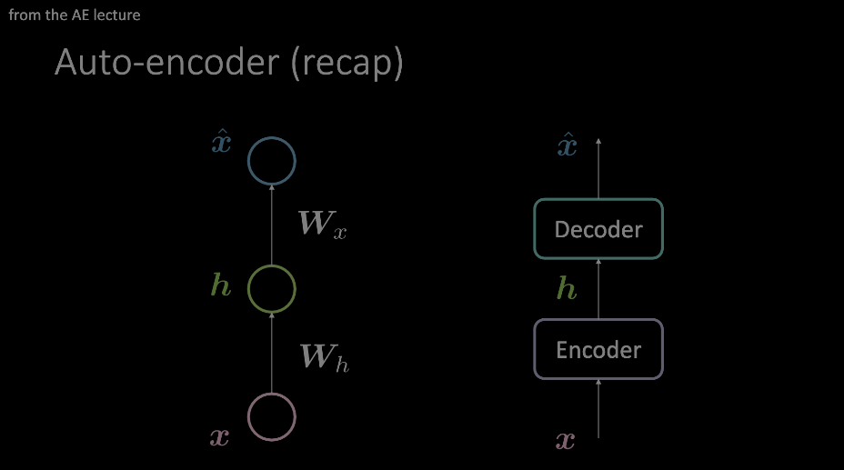
Figure 1: Two example diagrams of an autoencoder. The model on the left shows how an autoencoder can be design with two affine transformations + activations, where the image on the right replaces this single "layer" with an arbitrary module of operations.

Our “attention” is drawn to the autoencoder layout as shown in the model on the right and will now take a look inside, in the context of transformers.

Encoder Module

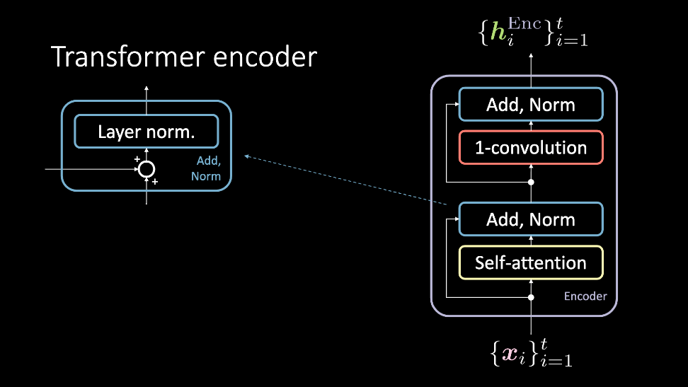
Figure 2: The transformer encoder, which accepts at set of inputs $\vect{x}$, and outputs a set of hidden representations $\vect{h}^\text{Enc}$.

The encoder module accepts a set of inputs, which are simultaneously fed through the self attention block and bypasses it to reach the Add, Norm block. At which point, they are again simultaneously passed through the 1D-Convolution and another Add, Norm block, and consequently outputted as the set of hidden representation. This set of hidden representation is then either sent through an arbitrary number of encoder modules i.e. more layers), or to the decoder. We shall now discuss these blocks in more detail.

Self-attention

The self-attention model is a normal attention model. The query, key, and value are generated from the same item of the sequential input. In tasks that try to model sequential data, positional encodings are added prior to this input. The output of this block is the attention-weighted values. The self-attention block accepts a set of inputs, from $1, \cdots , t$, and outputs $1, \cdots, t$ attention weighted values which are fed through the rest of the encoder.

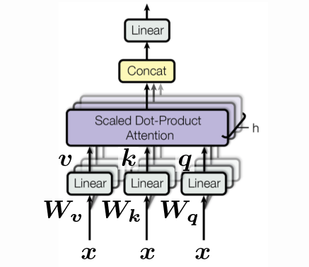
Figure 3: The self-attention block. The sequence of inputs is shown as a set along the 3rd dimension, and concatenated.

Add, Norm

The add norm block has two components. First is the add block, which is a residual connection, and layer normalization.

1D-convolution

Following this step, a 1D-convolution (aka a position-wise feed forward network) is applied. This block consists of two dense layers. Depending on what values are set, this block allows you to adjust the dimensions of the output $\vect{h}^\text{Enc}$.

Decoder Module

The transformer decoder follows a similar procedure as the encoder. However, there is one additional sub-block to take into account. Additionally, the inputs to this module are different.

Figure 4: A friendlier explanation of the decoder.

Cross-attention

The cross attention follows the query, key, and value setup used for the self-attention blocks. However, the inputs are a little more complicated. The input to the decoder is a data point $\vect{y}_i$, which is then passed through the self attention and add norm blocks, and finally ends up at the cross-attention block. This serves as the query for cross-attention, where the key and value pairs are the output $\vect{h}^\text{Enc}$, where this output was calculated with all past inputs $\vect{x}_1, \cdots, \vect{x}_{t}$.

Summary

A set, $\vect{x}_1$ to $\vect{x}_{t}$ is fed through the encoder. Using self-attention and some more blocks, an output representation, $\lbrace\vect{h}^\text{Enc}\rbrace_{i=1}^t$ is obtained, which is fed to the decoder. After applying self-attention to it, cross attention is applied. In this block, the query corresponds to a representation of a symbol in the target language $\vect{y}_i$, and the key and values are from the source language sentence ($\vect{x}_1$ to $\vect{x}_{t}$). Intuitively, cross attention finds which values in the input sequence are most relevant to constructing $\vect{y}_t$, and therefore deserve the highest attention coefficients. The output of this cross attention is then fed through another 1D-convolution sub-block, and we have $\vect{h}^\text{Dec}$. For the specified target language, it is straightforward from here to see how training will commence, by comparing $\lbrace\vect{h}^\text{Dec}\rbrace_{i=1}^t$ to some target data.

Word Language Models

There are a few important facts we left out before to explain the most important modules of a transformer, but will need to discuss them now to understand how transformers can achieve state-of-the-art results in language tasks.

Positional encoding

Attention mechanisms allow us to parallelize the operations and greatly accelerate a model’s training time, but loses sequential information. The positional encoding feature enables allows us to capture this context.

Semantic Representations

Throughout the training of a transformer, many hidden representations are generated. To create an embedding space similar to the one used by the word-language model example in PyTorch, the output of the cross-attention, will provide a semantic representation of the word $x_i$, at which point further experimentation can be performed over this dataset.

Code Summary

We will now see the blocks of transformers discussed above in a far more understandable format, code!

The first module we will look at the multi-headed attention block. Depending on query, key, and values entered into this block, it can either be used for self or cross attention.

class MultiHeadAttention(nn.Module):
    def __init__(self, d_model, num_heads, p, d_input=None):
        super().__init__()
        self.num_heads = num_heads
        self.d_model = d_model
        if d_input is None:
            d_xq = d_xk = d_xv = d_model
        else:
            d_xq, d_xk, d_xv = d_input
        # Embedding dimension of model is a multiple of number of heads
        assert d_model % self.num_heads == 0
        self.d_k = d_model // self.num_heads
        # These are still of dimension d_model. To split into number of heads
        self.W_q = nn.Linear(d_xq, d_model, bias=False)
        self.W_k = nn.Linear(d_xk, d_model, bias=False)
        self.W_v = nn.Linear(d_xv, d_model, bias=False)
        # Outputs of all sub-layers need to be of dimension d_model
        self.W_h = nn.Linear(d_model, d_model)

Initialization of multi-headed attention class. If a d_input is provided, this becomes cross attention. Otherwise, self-attention. The query, key, value setup is constructed as a linear transformation of the input d_model.

def scaled_dot_product_attention(self, Q, K, V):
    batch_size = Q.size(0)
    k_length = K.size(-2)

    # Scaling by d_k so that the soft(arg)max doesnt saturate
    Q = Q / np.sqrt(self.d_k)  # (bs, n_heads, q_length, dim_per_head)
    scores = torch.matmul(Q, K.transpose(2,3))  # (bs, n_heads, q_length, k_length)

    A = nn_Softargmax(dim=-1)(scores)  # (bs, n_heads, q_length, k_length)

    # Get the weighted average of the values
    H = torch.matmul(A, V)  # (bs, n_heads, q_length, dim_per_head)

    return H, A

Return hidden layer corresponding to encodings of values after scaled by the attention vector. For book-keeping purposes (which values in the sequence were masked out by attention?) A is also returned.

def split_heads(self, x, batch_size):
    return x.view(batch_size, -1, self.num_heads, self.d_k).transpose(1, 2)

Split the last dimension into (heads × depth). Return after transpose to put in shape (batch_size × num_heads × seq_length × d_k)

def group_heads(self, x, batch_size):
    return x.transpose(1, 2).contiguous().
        view(batch_size, -1, self.num_heads * self.d_k)

Combines the attention heads together, to get correct shape consistent with batch size and sequence length.

def forward(self, X_q, X_k, X_v):
    batch_size, seq_length, dim = X_q.size()
    # After transforming, split into num_heads
    Q = self.split_heads(self.W_q(X_q), batch_size)
    K = self.split_heads(self.W_k(X_k), batch_size)
    V = self.split_heads(self.W_v(X_v), batch_size)
    # Calculate the attention weights for each of the heads
    H_cat, A = self.scaled_dot_product_attention(Q, K, V)
    # Put all the heads back together by concat
    H_cat = self.group_heads(H_cat, batch_size)  # (bs, q_length, dim)
    # Final linear layer
    H = self.W_h(H_cat)  # (bs, q_length, dim)
    return H, A

The forward pass of multi headed attention.

Given an input is split into q, k, and v, at which point these values are fed through a scaled dot product attention mechanism, concatenated and fed through a final linear layer. The last output of the attention block is the attention found, and the hidden representation that is passed through the remaining blocks.

Although the next block shown in the transformer/encoder’s is the Add,Norm, which is a function already built into PyTorch. As such, it is an extremely simple implementation, and does not need it’s own class. Next is the 1-D convolution block. Please refer to previous sections for more details.

Now that we have all of our main classes built (or built for us), we now turn to an encoder module.

class EncoderLayer(nn.Module):
    def __init__(self, d_model, num_heads, conv_hidden_dim, p=0.1):
        self.mha = MultiHeadAttention(d_model, num_heads, p)
        self.layernorm1 = nn.LayerNorm(normalized_shape=d_model, eps=1e-6)
        self.layernorm2 = nn.LayerNorm(normalized_shape=d_model, eps=1e-6)

    def forward(self, x):
        attn_output, _ = self.mha(x, x, x)
        out1 = self.layernorm1(x + attn_output)
        cnn_output = self.cnn(out1)
        out2 = self.layernorm2(out1 + cnn_output)
        return out2

In the most powerful transformers, an arbitrarily large number of these encoders are stacked on top of one another.

Recall that self attention by itself does not have any recurrence or convolutions, but that’s what allows it to run so quickly. To make it sensitive to position we provide positional encodings. These are calculated as follows:

As to not take up too much room on the finer details, we will point you to https://github.com/Atcold/pytorch-Deep-Learning/blob/master/15-transformer.ipynb for the full code used here.

An entire encoder, with N stacked encoder layers, as well as position embeddings, is written out as

class Encoder(nn.Module):
    def __init__(self, num_layers, d_model, num_heads, ff_hidden_dim,
            input_vocab_size, maximum_position_encoding, p=0.1):
        self.embedding = Embeddings(d_model, input_vocab_size,
                                    maximum_position_encoding, p)
        self.enc_layers = nn.ModuleList()
        for _ in range(num_layers):
            self.enc_layers.append(EncoderLayer(d_model, num_heads,
                                                ff_hidden_dim, p))
    def forward(self, x):
        x = self.embedding(x) # Transform to (batch_size, input_seq_length, d_model)
        for i in range(self.num_layers):
            x = self.enc_layers[i](x)
        return x  # (batch_size, input_seq_len, d_model)

Example Use

There is a lot of tasks you can use just an Encoder for. In the accompanying notebook, we see how an encoder can be used for sentiment analysis.

Using the imdb review dataset, we can output from the encoder a latent representation of a sequence of text, and train this encoding process with binary cross entropy, corresponding to a positive or negative movie review.

Again we leave out the nuts and bolts, and direct you to the notebook, but here is the most important architectural components used in the transformer:

class TransformerClassifier(nn.Module):
    def forward(self, x):
        x = Encoder()(x)
        x = nn.Linear(d_model, num_answers)(x)
        return torch.max(x, dim=1)

model = TransformerClassifier(num_layers=1, d_model=32, num_heads=2,
                         conv_hidden_dim=128, input_vocab_size=50002, num_answers=2)

Where this model is trained in typical fashion.