Self-Supervised Learning - Pretext Tasks

Success story of supervision: Pre-training

In the past decade, one of the major success recipes for many different Computer Vision problems has been learning visual representations by performing supervised learning for ImageNet classification. And, using these learned representations, or learned model weights as initialization for other computer vision tasks, where a large quantum of labelled data might not be available.

However, getting annotations for a dataset of the magnitude of ImageNet is immensely time-consuming and expensive. Example: ImageNet labelling with 14M images took roughly 22 human years.

Because of this, the community started to look for alternate labelling processes, such as hashtags for social media images, GPS locations, or self-supervised approaches where the label is a property of the data sample itself.

But an important question that arises before looking for alternate labelling processes is:

How much labelled data can we get after all?

• If we search for all images with object-level category and bounding box annotations then there are roughly 1 million images.
• Now, if the constraint for bounding box coordinates is relaxed, the number of images available jumps to 14 million (approximately).
• However, if we consider all images available on the internet, there is a jump of 5 orders in the quantity of data available.
• And, then there is data apart from images, which requires other sensory input to capture or understand.

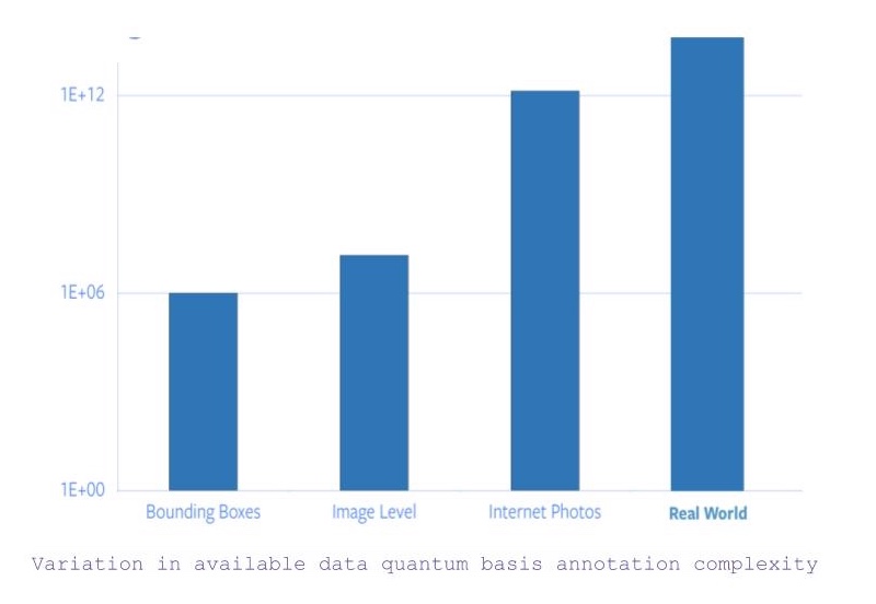
Figure 1: Variation in available data quantum basis complexity of annotation

Hence, drawing from the fact that ImageNet specific annotation alone took 22 human years worth of time, scaling labelling to all internet photos or beyond is completely infeasible.

Problem of Rare Concepts (Long Tail Problem)

Generally, the plot presenting distribution of the labels for internet images looks like a long tail. That is, most of the images correspond to very few labels, while there exist a large number of labels for which not many images are present. Thus, getting annotated samples for categories towards the end of the tail requires huge quantities of data to be labelled because of the nature of the distribution of categories.

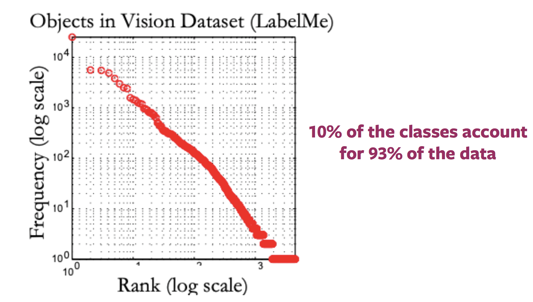
Figure 2: Variation in distribution of available images with labels

Problem of Different Domains

This method of ImageNet pre-training and fine-tuning on downstream task gets even murkier when the downstream task images belong to a completely different domain, such as medical imaging. And, obtaining a dataset of the quantum of ImageNet for pre-training for different domains is not possible.

What is self-supervised Learning?

Two ways to define self-supervised learning

• Basis supervised learning definition, i.e. the network follows supervised learning where labels are obtained in a semi-automated manner, without human input.
• Prediction problem, where a part of the data is hidden, and rest visible. Hence, the aim is to either predict the hidden data or to predict some property of the hidden data.

How self-supervised learning differs from supervised learning and unsupervised learning?

• Supervised learning tasks have pre-defined (and generally human-provided) labels,
• Unsupervised learning has just the data samples without any supervision, label or correct output.
• Self-supervised learning derives its labels from a co-occurring modality for the given data sample or from a co-occurring part of the data sample itself.

Self-Supervised Learning in Natural Language Processing

Word2Vec

• Given an input sentence, the task involves predicting a missing word from that sentence, which is specifically omitted for the purpose of building a pretext task.
• Hence, the set of labels becomes all possible words in the vocabulary, and, the correct label is the word that was omitted from the sentence.
• Thus, the network can then be trained using regular gradient-based methods to learn word-level representations.

Why self-supervised learning?

• Self-supervised learning enables learning representations of data by just observations of how different parts of the data interact.
• Thereby drops the requirement of huge amount of annotated data.
• Additionally, enables to leverage multiple modalities that might be associated with a single data sample.

Self-Supervised Learning in Computer Vision

Generally, computer vision pipelines that employ self-supervised learning involve performing two tasks, a pretext task and a real (downstream) task.

• The real (downstream) task can be anything like classification or detection task, with insufficient annotated data samples.
• The pretext task is the self-supervised learning task solved to learn visual representations, with the aim of using the learned representations or model weights obtained in the process, for the downstream task.

Developing pretext tasks

• Pretext tasks for computer vision problems can be developed using either images, video, or video and sound.
• In each pretext task, there is part visible and part hidden data, while the task is to predict either the hidden data or some property of the hidden data.

Example pretext tasks: Predicting relative position of image patches

• Input: 2 image patches, one is the anchor image patch while the other is the query image patch.
• Given the 2 image patches, the network needs to predict the relative position of the query image patch with respect to the anchor image patch.
• Thus, this problem can be modelled as an 8-way classification problem, since there are 8 possible locations for a query image, given an anchor.
• And, the label for this task can be automatically generated by feeding the relative position of query patch with respect to the anchor.

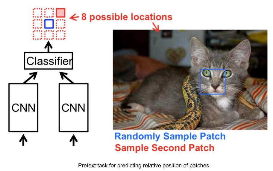
Figure 3: Relative Position task

Visual representations learned by relative position prediction task

We can evaluate the effectiveness of the learned visual representations by checking nearest neighbours for a given image patch basis feature representations provided by the network. For computing nearest neighbours of a given image patch,

• Compute the CNN features for all images in the dataset, that will act as the sample pool for retrieval.
• Compute CNN features for the required image patch.
• Identify nearest neighbours for the feature vector of the required image, from the pool of feature vectors of images available.

Relative position task finds out image patches that are very similar to the input image patch, while maintains invariance to factors such as object colour. Thus, the relative position task is able to learn visual representations, where representations for image patches with similar visual appearance are closer in the representation space as well.

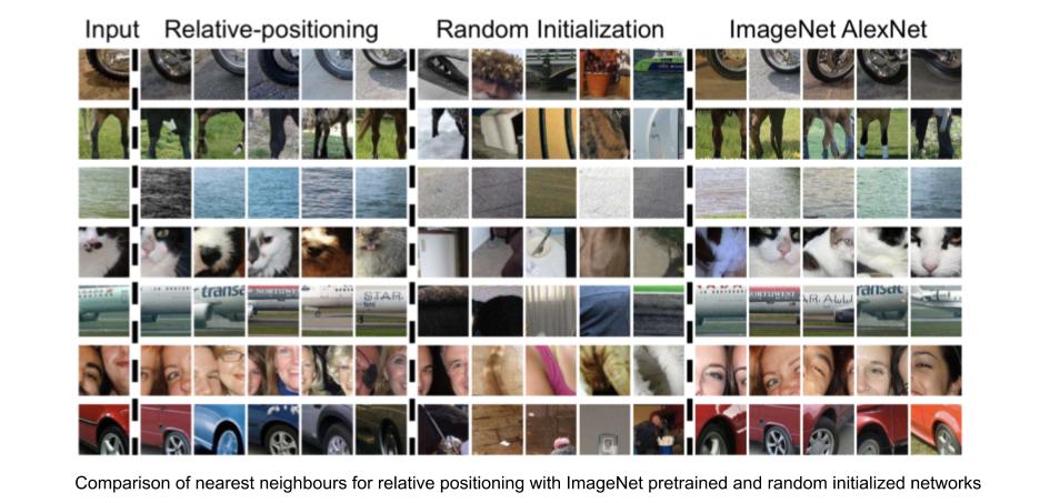
Figure 4: Relative Position: Nearest Neighbours

Predicting Rotation of Images

• Predicting rotations is one of the most popular pretext task which has a simple and straightforward architecture and requires minimal sampling.
• We apply rotations of 0, 90, 180, 270 degrees to the image and send these rotated images to the network to predict what sort of rotation was applied to the image and the network simply performs a 4-way classification to predict the rotation.
• Predicting rotations does not make any semantic sense, we are just using this pretext task as a proxy to learn some features and representations to be used in a downstream task.

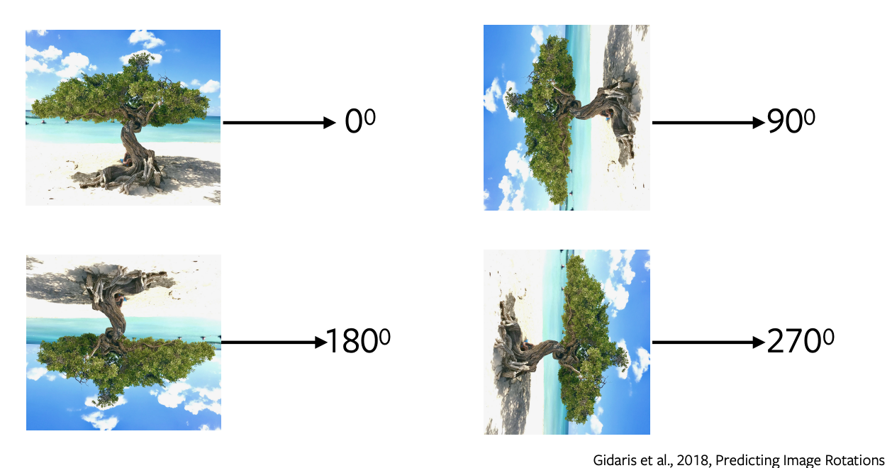
Figure 5: Rotations of Image

Why rotation helps or why it works?

It has been proven that it works empirically. The intuition behind it is that in order to predict the rotations, model needs to understand the rough boundaries and representation of an image. For example, it will have to segregate the sky from water or sand from the water or will understand that trees grow upwards and so on.

Colourisation

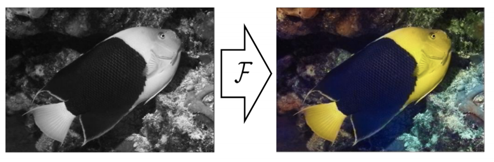
Figure 6: Colourisation

In this pretext task, we predict the colours of a grey image. It can be formulated for any image, we just remove the colour and feed this greyscale image to the network to predict its colour. This task is useful in some respects like for colourising the old greyscale films [//]: <> (we can apply this pretext task). The intuition behind this task is that the network needs to understand some meaningful information like that the trees are green, the sky is blue and so on.

It is important to note that colour mapping is not deterministic, and several possible true solutions exist. So, for an object if there are several possible colours then the network will colour it as grey which is the mean of all possible solutions. There have been recent works using Variational Auto Encoders and latent variables for diverse colourisation.

Fill in the blanks

We hide a part of an image and predict the hidden part from the remaining surrounding part of the image. This works because the network will learn the implicit structure of the data like to represent that cars run on roads, buildings are composed of windows & doors and so on.

Pretext Tasks for videos

Videos are composed of sequences of frames and this notion is the idea behind self-supervision, which can be leveraged for some pretext tasks like predicting the order of frames, fill in the blanks and object tracking.

Shuffle & Learn

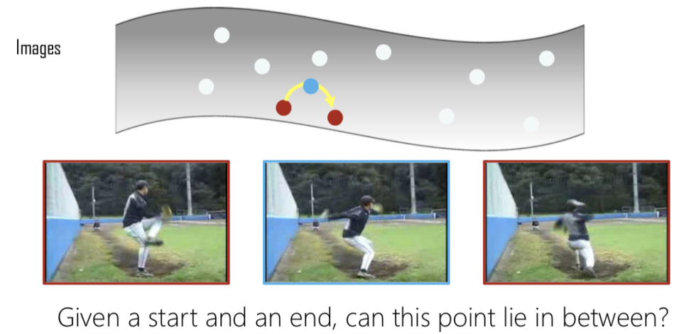
Figure 7: Interpolation

Given a bunch of frames, we extract three frames and if they are extracted in the right order we label it as positive, else if they are shuffled, label it as negative. This now becomes a binary classification problem to predict if the frames are in the right order or not. So, given a start and end point, we check if the middle is a valid interpolation of the two.

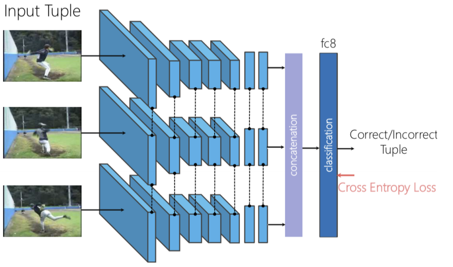
Figure 8: Shuffle & Learn architecture

We can use a triplet Siamese network, where the three frames are independently fed forward and then we concatenate the generated features and perform the binary classification to predict if the frames are shuffled or not.

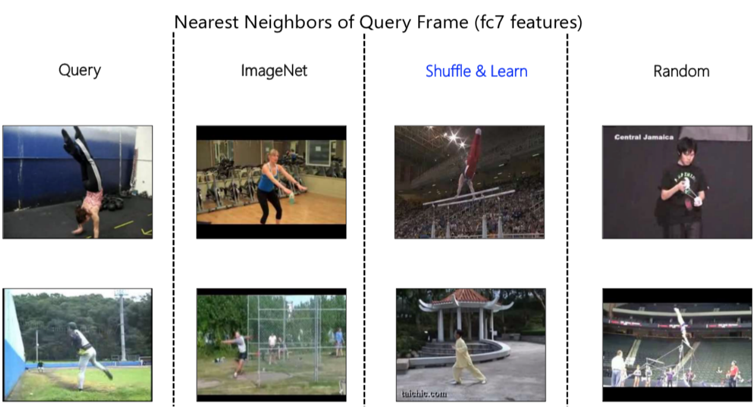
Figure 9: Nearest Neighbours Representation

Again, we can use the Nearest Neighbours algorithm to visualize what our networks are learning. In fig. 9 above, first we have a query frame which we feed-forward to get a feature representation and then look at the nearest neighbours in the representation space. While comparing, we can observe a stark difference between neighbours obtained from ImageNet, Shuffle & Learn and Random.

ImageNet is good at collapsing the entire semantic as it could figure out that it is a gym scene for the first input. Similarly, it could figure out that it is an outdoor scene with grass etc. for the second query. Whereas, when we observe Random we can see that it gives high importance to the background colour.

On observing Shuffle & Learn, it is not immediately clear whether it is focusing on the colour or on the semantic concept. After further inspection and observing various examples, it was observed that it is looking at the pose of the person. For example, in the first image the person is upside down and in second the feet are in a particular position similar to query frame, ignoring the scene or background colour. The reasoning behind this is that our pretext task was predicting whether the frames are in the right order or not, and to do this the network needs to focus on what is moving in the scene, in this case, the person.

It was verified quantitatively by fine-tuning this representation to the task of human key-point estimation, where given a human image we predict where certain key points like nose, left shoulder, right shoulder, left elbow, right elbow, etc. are. This method is useful for tracking and pose estimation.

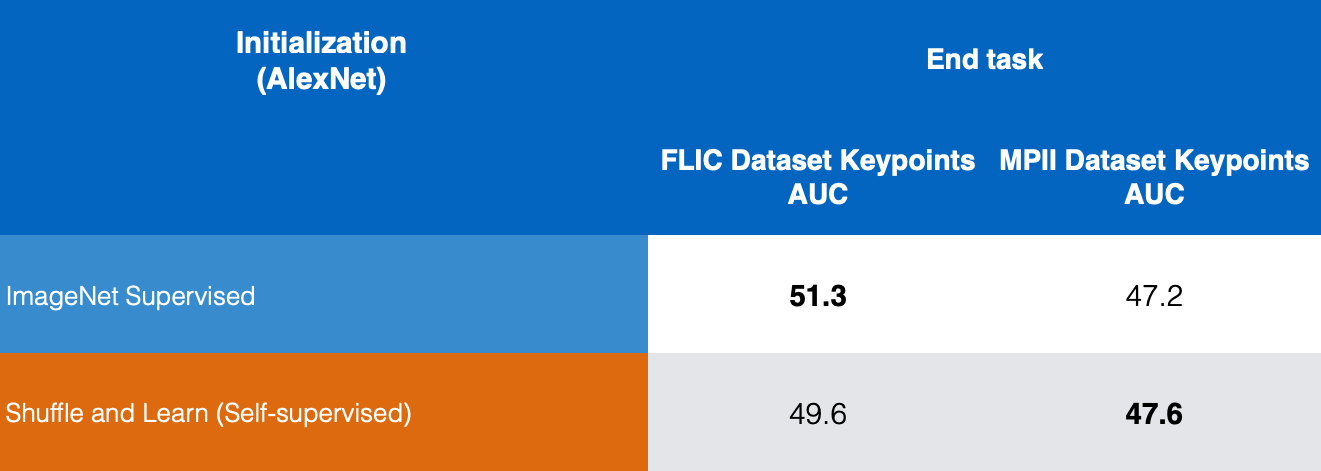
Figure 10: Key point Estimation comparison

In figure 10, we compare the results for supervised ImageNet and Self-Supervised Shuffle & Learn on FLIC and MPII datasets and we can see that Shuffle and Learn gives good results for key point estimation.

Pretext Tasks for videos and sound

Video and Sound are multi-modal where we have two modalities or sensory inputs one for video and one for sound. Where we try to predict whether the given video clip corresponds to the audio clip or not.

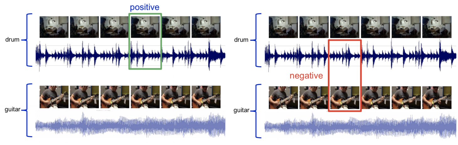
Figure 11: Video and sound sampling

Given a video with audio of a drum, sample the video frame with corresponding audio and call it a positive set. Next, take the audio of a drum and the video frame of a guitar and tag it as a negative set. Now we can train a network to solve this as a binary classification problem.

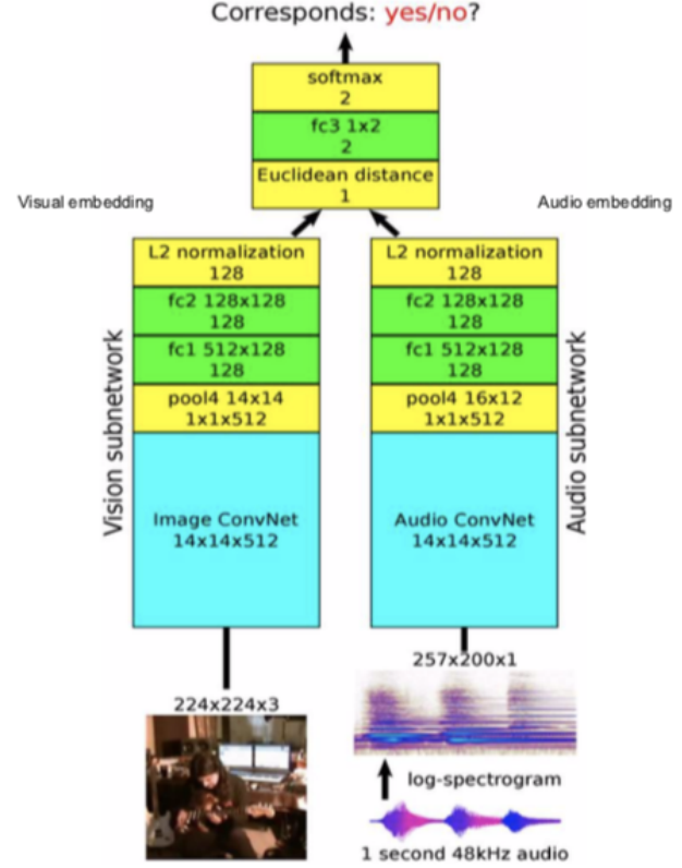
Figure 12: Architecture

Architecture: Pass the video frames to the vision subnetwork and pass the audio to the audio subnetwork, which gives 128-dimensional features and embeddings, we then fuse them together and solve it as a binary classification problem predicting if they correspond with each other or not.

It can be used to predict what in the frame might be making a sound. The intuition is if it is the sound of a guitar, the network roughly needs to understand how the guitar looks and same should be true for drums.

Understanding what the “pretext” task learns

• Pretext tasks should be complementary

  • Let’s take for example the pretext tasks Relative Position and Colourisation. We can boost performance by training a model to learn both pretext tasks as shown below:

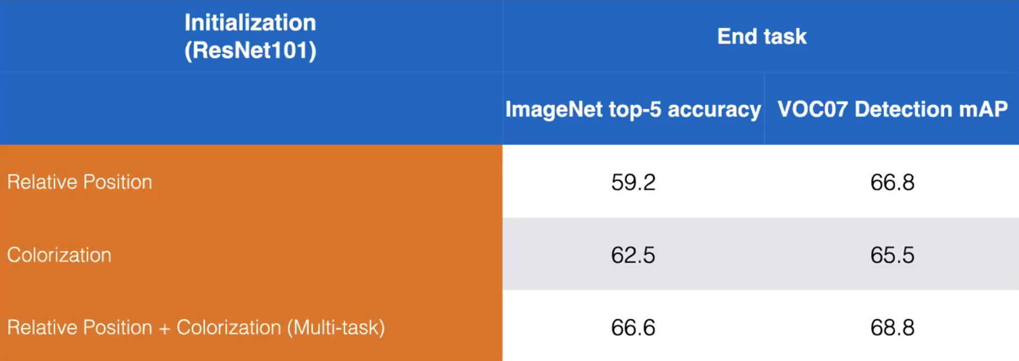
Figure 13: Comparison of disjoint *vs.* combined training of Relative Position and Colourisation pretext tasks. ResNet101. (Misra)

• A single pretext task may not be the right answer to learn SS representations

• Pretext tasks vary greatly in what they try to predict (difficultly)

  • Relative position is easy since it’s a simple classification
  • Masking and fill-in is far harder –> better representation
  • Contrastive methods generate even more info than pretext tasks

• Question: How do we train multiple pre-training tasks?

  • The pretext output will depend on the input. The final fully-connected layer of the network can be swapped depending on the batch type.
  • For example: A batch of black-and-white images is fed to the network in which the model is to produce a coloured image. Then, the final layer is switched, and given a batch of patches to predict relative position.

• Question: How much should we train on a pretext task?

• Rule of thumb: Have a very difficult pretext task such that it improves the downstream task.
• In practice, the pretext task is trained, and may not be re-trained. In development, it is trained as part of the entire pipeline.

Scaling Self-Supervised Learning

Jigsaw Puzzles

• Partition an image into multiple tiles and then shuffle these tiles. The model is then tasked with un-shuffling the tiles back to the original configuration. (Noorozi & Favaro, 2016)

  • Predict which permutation was applied to the input
  • This is done by creating batches of tiles such that each tile of an image is evaluated independently. The convolution output are then concatenated and the permutation is predicted as in figure below

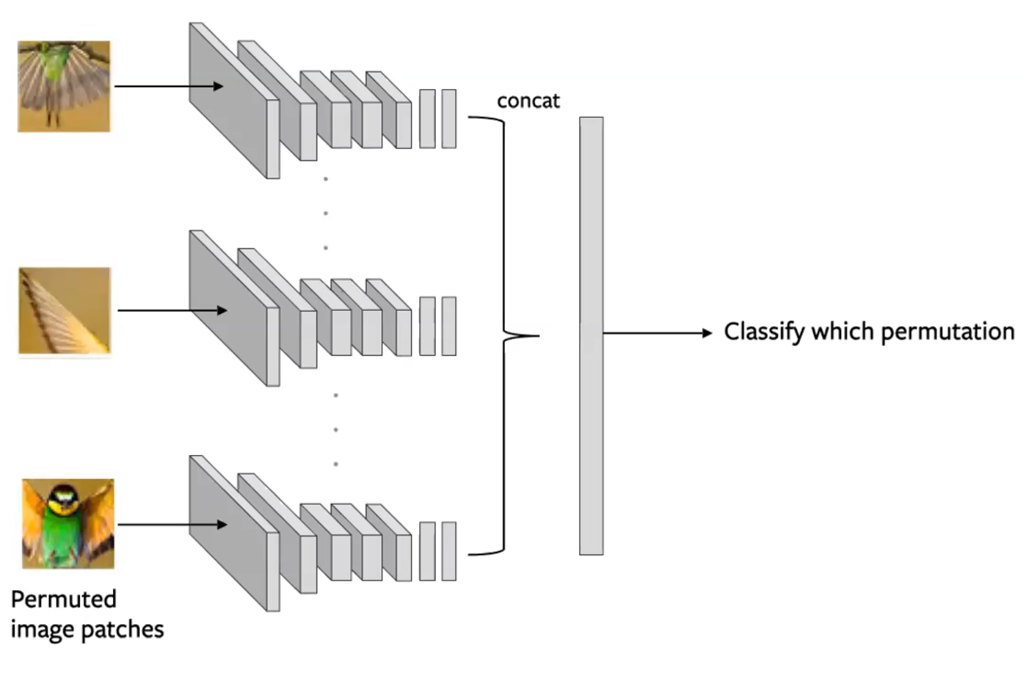
Figure 14: Siamese network architecture for a Jigsaw pretext task. Each tile is passed through independently, with encodings concatenated to predict a permutation. (Misra)

• Considerations:
  1. Use a subset of permutations i.e. From 9!, use 100)
  2. The n-way ConvNet uses shared parameters
  3. The problem complexity is the size of the subset. The amount of information you are predicting.

• Sometimes, this method can perform better on downstream tasks than supervised methods, since the network is able to learn some concepts about the geometry of its input.

• Shortcomings: Few Shot Learning: Limited number of training examples

  • Self-supervised representations are not as sample efficient

Evaluation: Fine-tuning vs. Linear Classifier

This form of evaluation is a kind of Transfer Learning.

• Fine Tuning: When applying to our downstream task, we use our entire network as an initialization for which to train a new one, updating all the weights.

• Linear Classifier: On top of our pretext network, we train a small linear classifier to perform our downstream task, leaving the rest of the network intact.

A good representation should transfer with a little training.

• It is helpful to evaluate the pretext learning on a multitude of different tasks. We can do so by extracting the representation created by different layers in the network as fixed features and evaluating their usefulness across these different tasks.
  • Measurement: Mean Average Precision (mAP) –The precision averaged across all the different tasks we are considering.
  • Some examples of these tasks include: Object Detection (using fine-tuning), Surface Normal Estimation (see NYU-v2 dataset)
• What does each layer learn?
  • Generally, as the layers become deeper, the mean average precision on downstream tasks using their representations will increase.
  • However, the final layer will see a sharp drop in the mAP due to the layer becoming overly specialized.
    • This contrasts with supervised networks, in that the mAP generally always increases with depth of layer.
    • This shows that the pretext task is not well-aligned to the downstream task.