Linear Algebra and Convolutions

🎙️ Alfredo Canziani

Linear Algebra review

This part is a recap of basic linear algebra in the context of neural networks. We start with a simple hidden layer $\boldsymbol{h}$:

\[\boldsymbol{h} = f(\boldsymbol{z})\]

The output is a non-linear function $f$ applied to a vector $z$. Here $z$ is the output of an affine transformation $\boldsymbol{A} \in\mathbb{R^{m\times n}}$ to the input vector $\boldsymbol{x} \in\mathbb{R^n}$:

\[\boldsymbol{z} = \boldsymbol{A} \boldsymbol{x}\]

For simplicity biases are ignored. The linear equation can be expanded as:

\[\boldsymbol{A}\boldsymbol{x} = \begin{pmatrix} a_{11} & a_{12} & \cdots & a_{1n}\\ a_{21} & a_{22} & \cdots & a_{2n} \\ \vdots & \vdots & \ddots & \vdots \\ a_{m1} & a_{m2} & \cdots & a_{mn} \end{pmatrix} \begin{pmatrix} x_1 \\ \vdots \\x_n \end{pmatrix} = \begin{pmatrix} \text{---} \; \boldsymbol{a}^{(1)} \; \text{---} \\ \text{---} \; \boldsymbol{a}^{(2)} \; \text{---} \\ \vdots \\ \text{---} \; \boldsymbol{a}^{(m)} \; \text{---} \\ \end{pmatrix} \begin{matrix} \rvert \\ \boldsymbol{x} \\ \rvert \end{matrix} = \begin{pmatrix} {\boldsymbol{a}}^{(1)} \boldsymbol{x} \\ {\boldsymbol{a}}^{(2)} \boldsymbol{x} \\ \vdots \\ {\boldsymbol{a}}^{(m)} \boldsymbol{x} \end{pmatrix}_{m \times 1}\]

where $\boldsymbol{a}^{(i)}$ is the $i$-th row of the matrix $\boldsymbol{A}$.

To understand the meaning of this transformation, let us analyse one component of $\boldsymbol{z}$ such as $a^{(1)}\boldsymbol{x}$. Let $n=2$, then $\boldsymbol{a} = (a_1,a_2)$ and $\boldsymbol{x} = (x_1,x_2)$.

$\boldsymbol{a}$ and $\boldsymbol{x}$ can be drawn as vectors in the 2D coordinate axis. Now, if the angle between $\boldsymbol{a}$ and $\hat{\boldsymbol{\imath}}$ is $\alpha$ and the angle between $\boldsymbol{x}$ and $\hat{\boldsymbol{\imath}}$ is $\xi$, then with trigonometric formulae $a^\top\boldsymbol{x}$ can be expanded as:

\[\begin {aligned} \boldsymbol{a}^\top\boldsymbol{x} &= a_1x_1+a_2x_2\\ &=\lVert \boldsymbol{a} \rVert \cos(\alpha)\lVert \boldsymbol{x} \rVert \cos(\xi) + \lVert \boldsymbol{a} \rVert \sin(\alpha)\lVert \boldsymbol{x} \rVert \sin(\xi)\\ &=\lVert \boldsymbol{a} \rVert \lVert \boldsymbol{x} \rVert \big(\cos(\alpha)\cos(\xi)+\sin(\alpha)\sin(\xi)\big)\\ &=\lVert \boldsymbol{a} \rVert \lVert \boldsymbol{x} \rVert \cos(\xi-\alpha) \end {aligned}\]

The output measures the alignment of the input to a specific row of the matrix $\boldsymbol{A}$. This can be understood by observing the angle between the two vectors, $\xi-\alpha$. When $\xi = \alpha$, the two vectors are perfectly aligned and maximum is attained. If $\xi - \alpha = \pi$, then $\boldsymbol{a}^\top\boldsymbol{x}$ attains its minimum and the two vectors are pointing at opposite directions. In essence, the linear transformation allows one to see the projection of an input to various orientations as defined by $A$. This intuition is expandable to higher dimensions as well.

Another way to understand the linear transformation is by understanding that $\boldsymbol{z}$ can also be expanded as:

\[\boldsymbol{A}\boldsymbol{x} = \begin{pmatrix} \vert & \vert & & \vert \\ \boldsymbol{a}_1 & \boldsymbol{a}_2 & \cdots & \boldsymbol{a}_n \\ \vert & \vert & & \vert \\ \end{pmatrix} \begin{matrix} \rvert \\ \boldsymbol{x} \\ \rvert \end{matrix} = x_1 \begin{matrix} \rvert \\ \boldsymbol{a}_1 \\ \rvert \end{matrix} + x_2 \begin{matrix} \rvert \\ \boldsymbol{a}_2 \\ \rvert \end{matrix} + \cdots + x_n \begin{matrix} \rvert \\ \boldsymbol{a}_n \\ \rvert \end{matrix}\]

The output is the weighted sum of the columns of matrix $\boldsymbol{A}$. Therefore, the signal is nothing but a composition of the input.

Extend Linear Algebra to convolutions

Now we extend linear algebra to convolutions, by using the example of audio data analysis. We start with representing a fully connected layer as a form of matrix multiplication: -

\[\begin{bmatrix} w_{11} & w_{12} & w_{13}\\ w_{21} & w_{22} & w_{23}\\ w_{31} & w_{32} & w_{33}\\ w_{41} & w_{42} & w_{43} \end{bmatrix} \begin{bmatrix} x_1\\ x_2\\ x_3 \end{bmatrix} = \begin{bmatrix} y_1\\ y_2\\ y_3\\ y_4 \end{bmatrix}\]

In this example, the weight matrix has a size of $4 \times 3$, the input vector has a size of $3 \times 1$ and the output vector has a of size $4 \times 1$.

However, for audio data, the data is much longer (not 3-sample long). The number of samples in the audio data is equal to the duration of the audio (e.g. 3 seconds) times the sampling rate (e.g. 22.05 kHz). As shown below, the input vector $\boldsymbol{x}$ will be quite long. Correspondingly, the weight matrix will become “fat”.

\[\begin{bmatrix} w_{11} & w_{12} & w_{13} & w_{14} & \cdots &w_{1k}& \cdots &w_{1n}\\ w_{21} & w_{22} & w_{23}& w_{24} & \cdots & w_{2k}&\cdots &w_{2n}\\ w_{31} & w_{32} & w_{33}& w_{34} & \cdots & w_{3k}&\cdots &w_{3n}\\ w_{41} & w_{42} & w_{43}& w_{44} & \cdots & w_{4k}&\cdots &w_{4n} \end{bmatrix} \begin{bmatrix} x_1\\ x_2\\ x_3\\ x_4\\ \vdots\\ x_k\\ \vdots\\ x_n \end{bmatrix} = \begin{bmatrix} y_1\\ y_2\\ y_3\\ y_4 \end{bmatrix}\]

The above formulation will be difficult to train. Fortunately there are ways to simplify the same.

Property: locality

Due to locality (i.e. we do not care for data points that are far away) of data, $w_{1k}$ from the weight matrix above, can be filled with 0 when $k$ is relatively large. Therefore, the first row of the matrix becomes a kernel of size 3. Let’s denote this size-3 kernel as $\boldsymbol{a}^{(1)} = \begin{bmatrix} a_1^{(1)} & a_2^{(1)} & a_3^{(1)} \end{bmatrix}$.

\[\begin{bmatrix} a_1^{(1)} & a_2^{(1)} & a_3^{(1)} & 0 & \cdots &0& \cdots &0\\ w_{21} & w_{22} & w_{23}& w_{24} & \cdots & w_{2k}&\cdots &w_{2n}\\ w_{31} & w_{32} & w_{33}& w_{34} & \cdots & w_{3k}&\cdots &w_{3n}\\ w_{41} & w_{42} & w_{43}& w_{44} & \cdots & w_{4k}&\cdots &w_{4n} \end{bmatrix} \begin{bmatrix} x_1\\ x_2\\ x_3\\ x_4\\ \vdots\\ x_k\\ \vdots\\ x_n \end{bmatrix} = \begin{bmatrix} y_1\\ y_2\\ y_3\\ y_4 \end{bmatrix}\]

Property: stationarity

Natural data signals have the property of stationarity (i.e. certain patterns/motifs will repeat). This helps us reuse kernel $\mathbf{a}^{(1)}$ that we defined previously. We use this kernel by placing it one step further each time (i.e. stride is 1), resulting in the following:

\[\begin{bmatrix} a_1^{(1)} & a_2^{(1)} & a_3^{(1)} & 0 & 0 & 0 & 0&\cdots &0\\ 0 & a_1^{(1)} & a_2^{(1)} & a_3^{(1)} & 0&0&0&\cdots &0\\ 0 & 0 & a_1^{(1)} & a_2^{(1)} & a_3^{(1)} & 0&0&\cdots &0\\ 0 & 0 & 0& a_1^{(1)} & a_2^{(1)} &a_3^{(1)} &0&\cdots &0\\ 0 & 0 & 0& 0 & a_1^{(1)} &a_2^{(1)} &a_3^{(1)} &\cdots &0\\ \vdots&&\vdots&&\vdots&&\vdots&&\vdots \end{bmatrix} \begin{bmatrix} x_1\\ x_2\\ x_3\\ x_4\\ \vdots\\ x_k\\ \vdots\\ x_n \end{bmatrix}\]

Both the upper right part and lower left part of the matrix are filled with $0$s thanks to locality, leading to sparsity. The reuse of a certain kernel again and again is called weight sharing.

Multiple layers of Toeplitz matrix

After these changes, the number of parameters we are left with is 3 (i.e. $a_1,a_2,a_3$). In comparison to the previous weight matrix, which had 12 parameters (i.e. $w_{11},w_{12},\cdots,w_{43}$), the current number of parameters is too restrictive and we would like to expand the same.

The previous matrix can be considered to be a layer (i.e. a convolutional layer) with the kernel $\boldsymbol{a}^{(1)}$. Then we can construct multiple layers with different kernels $\boldsymbol{a}^{(2)}$, $\boldsymbol{a}^{(3)}$, etc, thereby increasing the parameters.

Each layer has a matrix containing just one kernel that is replicated multiple times. This type of matrix is called a Toeplitz matrix. In every Toeplitz matrix, each descending diagonal from left to right is constant. The Toeplitz matrices that we use here are sparse matrices as well.

Given the first kernel $\boldsymbol{a}^{(1)}$ and the input vector $\boldsymbol{x}$, the first entry in the output given by this layer is, $a_1^{(1)} x_1 + a_2^{(1)} x_2 + a_3^{(1)}x_3$. Therefore, the whole output vector looks like the following: -

\[\begin{bmatrix} \mathbf{a}^{(1)}x[1:3]\\ \mathbf{a}^{(1)}x[2:4]\\ \mathbf{a}^{(1)}x[3:5]\\ \vdots \end{bmatrix}\]

The same matrix multiplication method can be applied on following convolutional layers with other kernels (e.g. $\boldsymbol{a}^{(2)}$ and $\boldsymbol{a}^{(3)}$) to get similar results.

Listening to convolutions - Jupyter Notebook

The Jupyter Notebook can be found here.

In this notebook, we are going to explore Convolution as a ‘running scalar product’.

The library librosa enables us to load the audio clip $\boldsymbol{x}$ and its sampling rate. In this case, there are 70641 samples, sampling rate is 22.05kHz and total length of the clip is 3.2s. The imported audio signal is wavy (refer to Fig 1) and we can guess what it sounds like from the amplitude of $y$ axis. The audio signal $x(t)$ is actually the sound played when turning off the Windows system (refer to Fig 2).

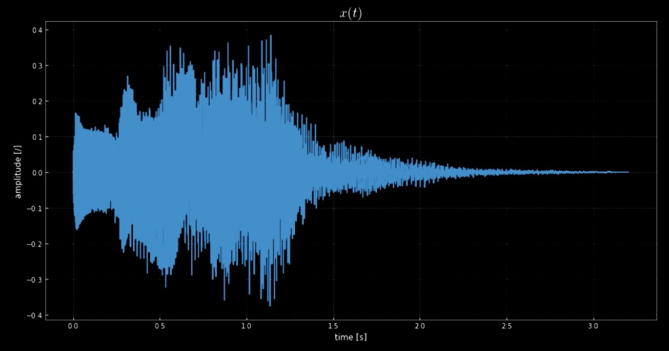
Fig. 1: A visualization of the audio signal.

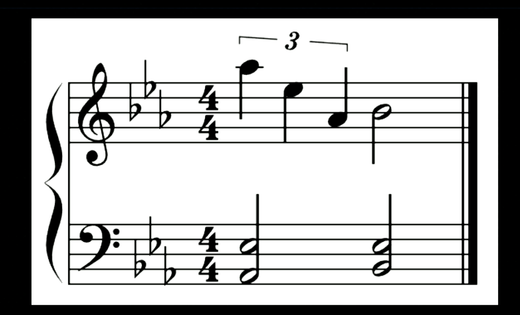
Fig. 2: Notes for the above audio signal.

We need to seperate the notes from the waveform. To achieve this, if we use Fourier transform (FT) all the notes would come out together and it will be hard to figure out the exact time and location of each pitch. Therefore, a localized FT is needed (also known as spectrogram). As is observed in the spectrogram (refer to Fig 3), different pitches peak at different frequencies (e.g. first pitch peaks at 1600). Concatenating the four pitches at their frequencies gives us a pitched version of the original signal.

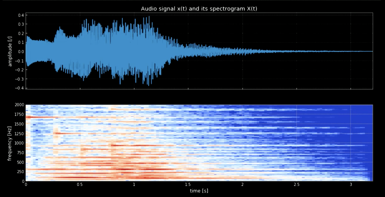
Fig. 3: Audio signal and its spectrogram.

Convolution of the input signal with all the pitches (all the keys of the piano for example) can help extract all notes in the input piece (i.e. the hits when the audio matches the specific kernels). The spectrograms of the original signal and the signal of the concatenated pitches is shown in Fig 4 while the frequencies of the original signal and the four pitches is shown in Fig 5. The plot of the convolutions of the four kernels with the input signal (original signal) is shown in Fig 6. Fig 6 along with the audio clips of the convolutions prove the effectiveness of the convolutions in extracting the notes.

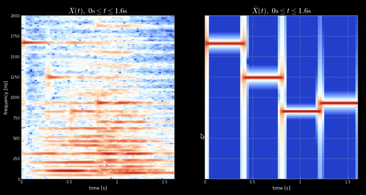
Fig. 4: Spectrogram of original signal (left) and Sepctrogram of the concatenation of pitches (right).

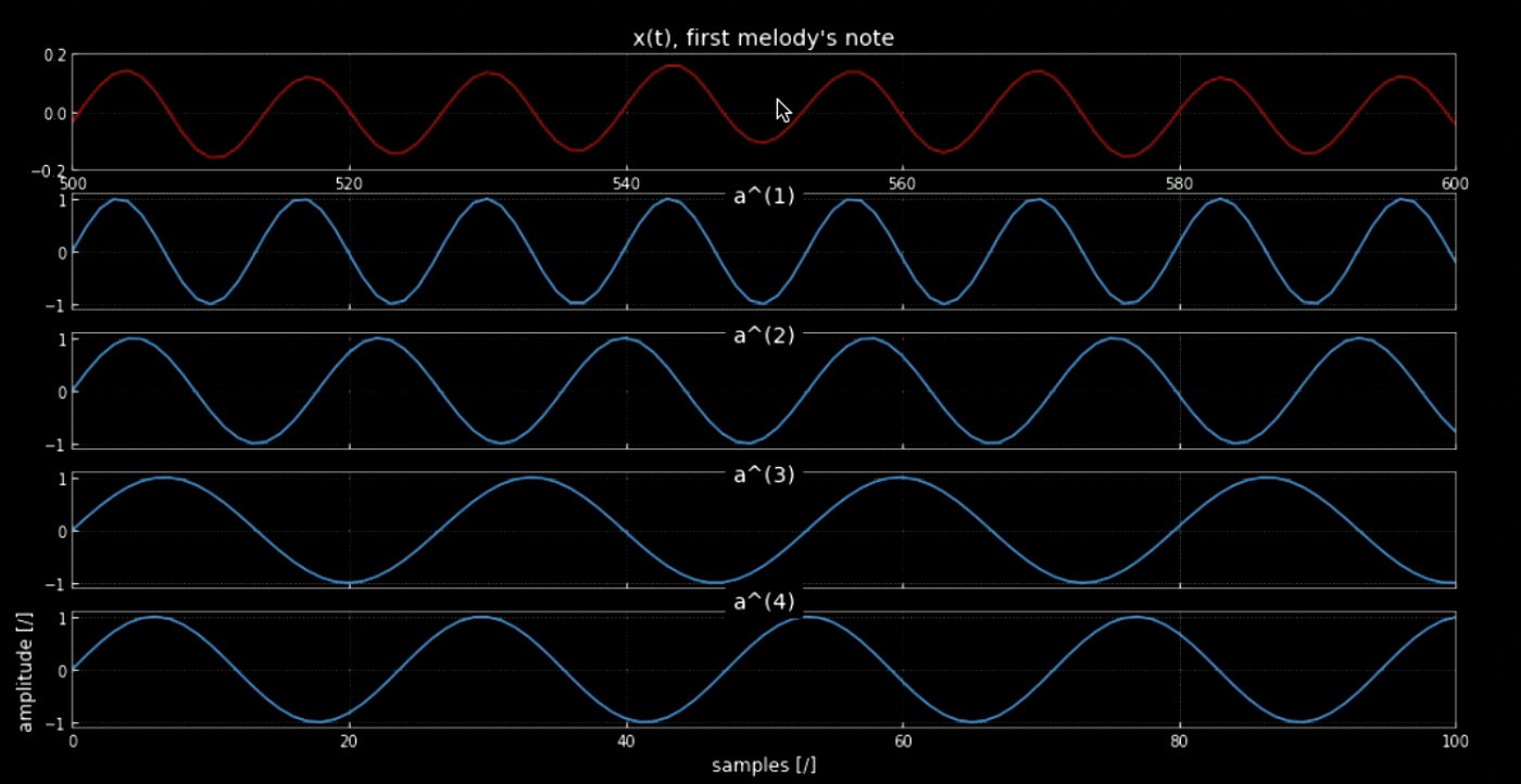
Fig. 5: First note of the melody.

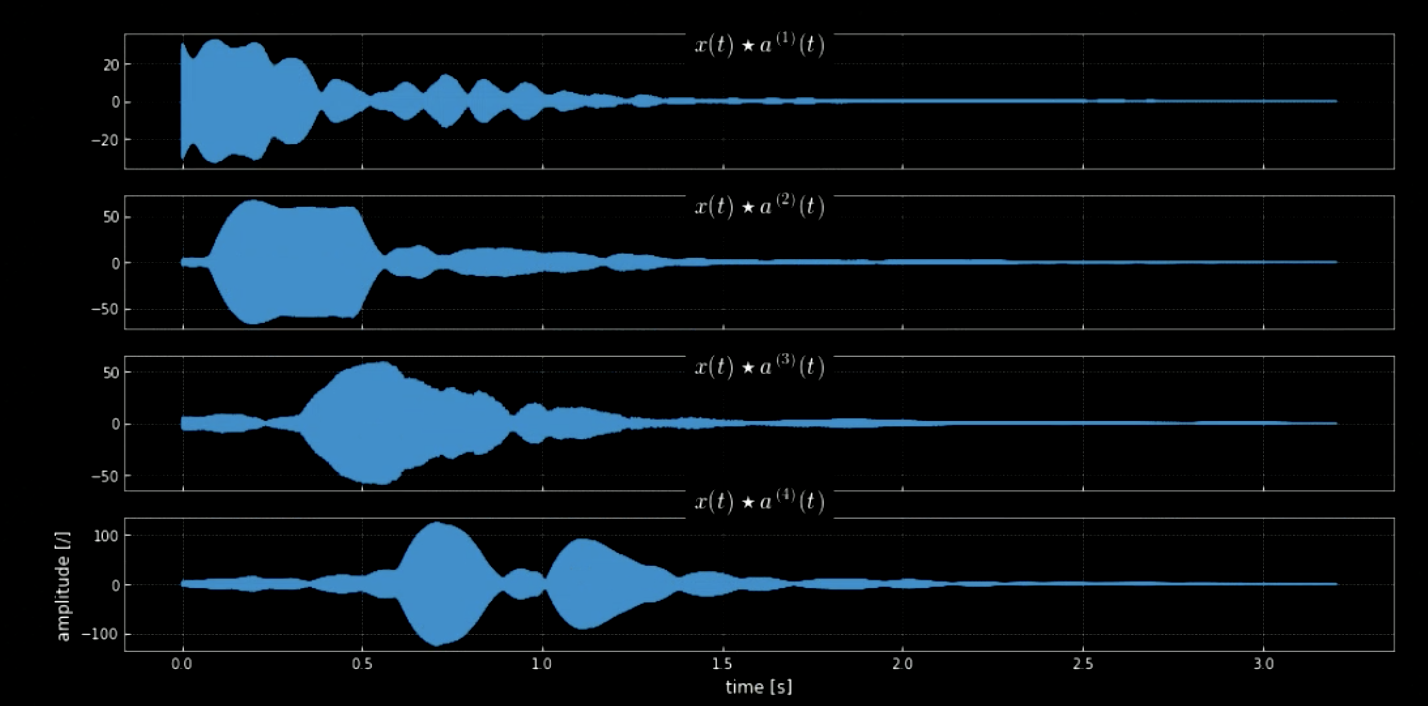
Fig. 6: Convolution of four kernels.

Dimensionality of different datasets

The last part is a short digression on the different representations of dimensionality and examples for the same. Here we consider input set $X$ is made of functions mapping from domains $\Omega$ to channels $c$.

Examples

• Audio data: domain is 1-D, discrete signal indexed by time; number of channels $c$ can range from 1 (mono), 2 (stereo), 5+1 (Dolby 5.1), etc.
• Image data: domain is 2-D (pixels); $c$ can range from 1(greyscale), 3(colour), 20(hyperspectral), etc.
• Special relativity: domain is $\mathbb{R^4} \times \mathbb{R^4}$ (space-time $\times$ four-momentum); when $c = 1$ it is called Hamiltonian.

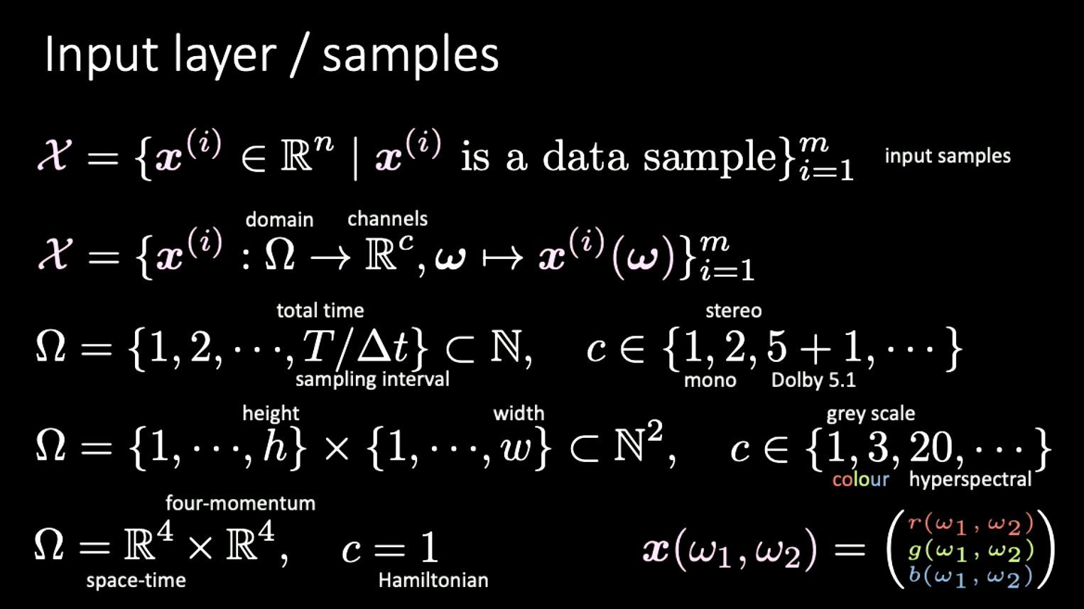
Fig. 7: Different dimensions of different types of signals.

---

📝 Yuchi Ge, Anshan He, Shuting Gu, and Weiyang Wen
18 Feb 2020