Architecture of RNN and LSTM Model

Overview

RNN is one type of architecture that we can use to deal with sequences of data. What is a sequence? From the CNN lesson, we learned that a signal can be either 1D, 2D or 3D depending on the domain. The domain is defined by what you are mapping from and what you are mapping to. Handling sequential data is basically dealing with 1D data since the domain is the temporal axis. Nevertheless, you can also use RNN to deal with 2D data, where you have two directions.

Vanilla vs. Recurrent NN

Figure 1 is a vanilla neural network diagram with three layers. “Vanilla” is an American term meaning plain. The pink bubble is the input vector x, in the center is the hidden layer in green, and the final blue layer is the output. Using an example from digital electronics on the right, this is like a combinational logic, where the current output only depends on the current input.

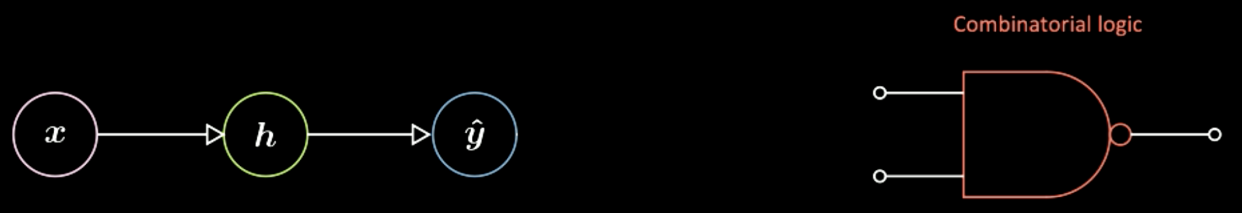
Figure 1: Vanilla Architecture

In contrast to a vanilla neural network, in recurrent neural networks the current output depends not only on the current input but also on the state of the system, shown in Figure 2. This is like a sequential logic in digital electronics, where the output also depends on a “flip-flop” (a basic memory unit in digital electronics). Therefore the main difference here is that the output of a vanilla neural network only depends on the current input, while the one of RNN depends also on the state of the system.

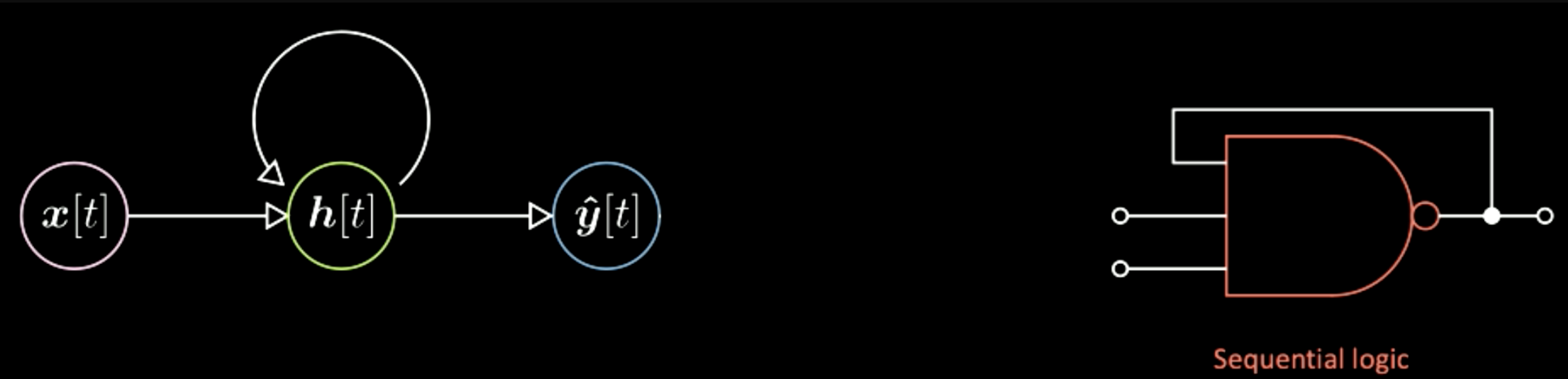
Figure 2: RNN Architecture

Figure 3: Basic NN Architecture

Yann’s diagram adds these shapes between neurons to represent the mapping between one tensor and another(one vector to another). For example, in Figure 3, the input vector x will map through this additional item to the hidden representations h. This item is actually an affine transformation i.e. rotation plus distortion. Then through another transformation, we get from the hidden layer to the final output. Similarly, in the RNN diagram, you can have the same additional items between neurons.

Figure 4: Yann's RNN Architecture

Four types of RNN Architectures and Examples

The first case is vector to sequence. The input is one bubble and then there will be evolutions of the internal state of the system annotated as these green bubbles. As the state of the system evolves, at every time step there will be one specific output.

Figure 5: Vec to Seq

An example of this type of architecture is to have the input as one image while the output will be a sequence of words representing the English descriptions of the input image. To explain using Figure 6, each blue bubble here can be an index in a dictionary of English words. For instance, if the output is the sentence “This is a yellow school bus”. You first get the index of the word “This” and then get the index of the word “is” and so on. Some of the results of this network are shown below. For example, in the first column the description regarding the last picture is “A herd of elephants walking across a dry grass field.”, which is very well refined. Then in the second column, the first image outputs “Two dogs play in the grass.”, while it’s actually three dogs. In the last column are the more wrong examples such as “A yellow school bus parked in a parking lot.” In general, these results show that this network can fail quite drastically and perform well sometimes. This is the case that is from one input vector, which is the representation of an image, to a sequence of symbols, which are for example characters or words making up the English sentences. This kind of architecture is called an autoregressive network. An autoregressive network is a network which gives an output given that you feed as input the previous output.

Figure 6: vec2seq Example: Image to Text

The second type is sequence to a final vector. This network keeps feeding a sequence of symbols and only at the end gives a final output. An application of this can be using the network to interpret Python. For example, the input are these lines of Python program.

Figure 7: Seq to Vec

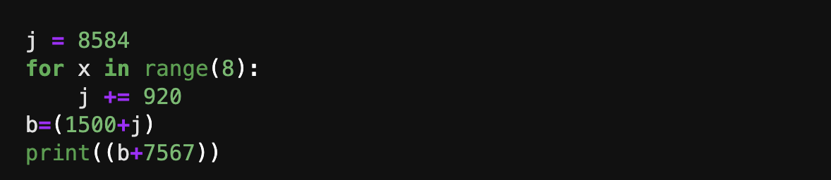
Figure 8: Input lines of Python Codes

Then the network will be able to output the correct solution of this program. Another more complicated program like this:

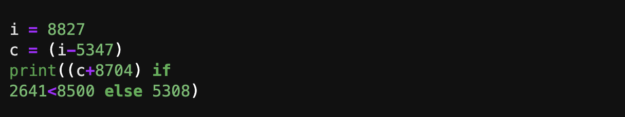
Figure 9: Input lines of Python Codes in a more Completed Case

Then the output should be 12184. These two examples display that you can train a neural network to do this kind of operation. We just need to feed a sequence of symbols and enforce the final output to be a specific value.

The third is sequence to vector to sequence, shown in Figure 10. This architecture used to be the standard way of performing language translation. You start with a sequence of symbols here shown in pink. Then everything gets condensed into this final h, which represents a concept. For instance, we can have a sentence as input and squeeze it temporarily into a vector, which is representing the meaning and message that to send across. Then after getting this meaning in whatever representation, the network unrolls it back into a different language. For example “Today I’m very happy” in a sequence of words in English can be translated into Italian or Chinese. In general, the network gets some kind of encoding as inputs and turns them into a compressed representation. Finally, it performs the decoding given the same compressed version. In recent times we have seen networks like Transformers, which we will cover in the next lesson, outperform this method at language translation tasks. This type of architecture used to be the state of the art about two years ago (2018).

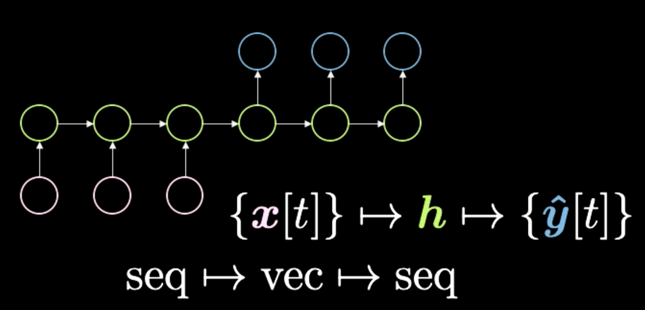
Figure 10: Seq to Vec to Seq

If you do a PCA over the latent space, you will have the words grouped by semantics like shown in this graph.

Figure 11: Words Grouped by Semantics after PCA

If we zoom in, we will see that the in the same location there are all the months, like January and November.

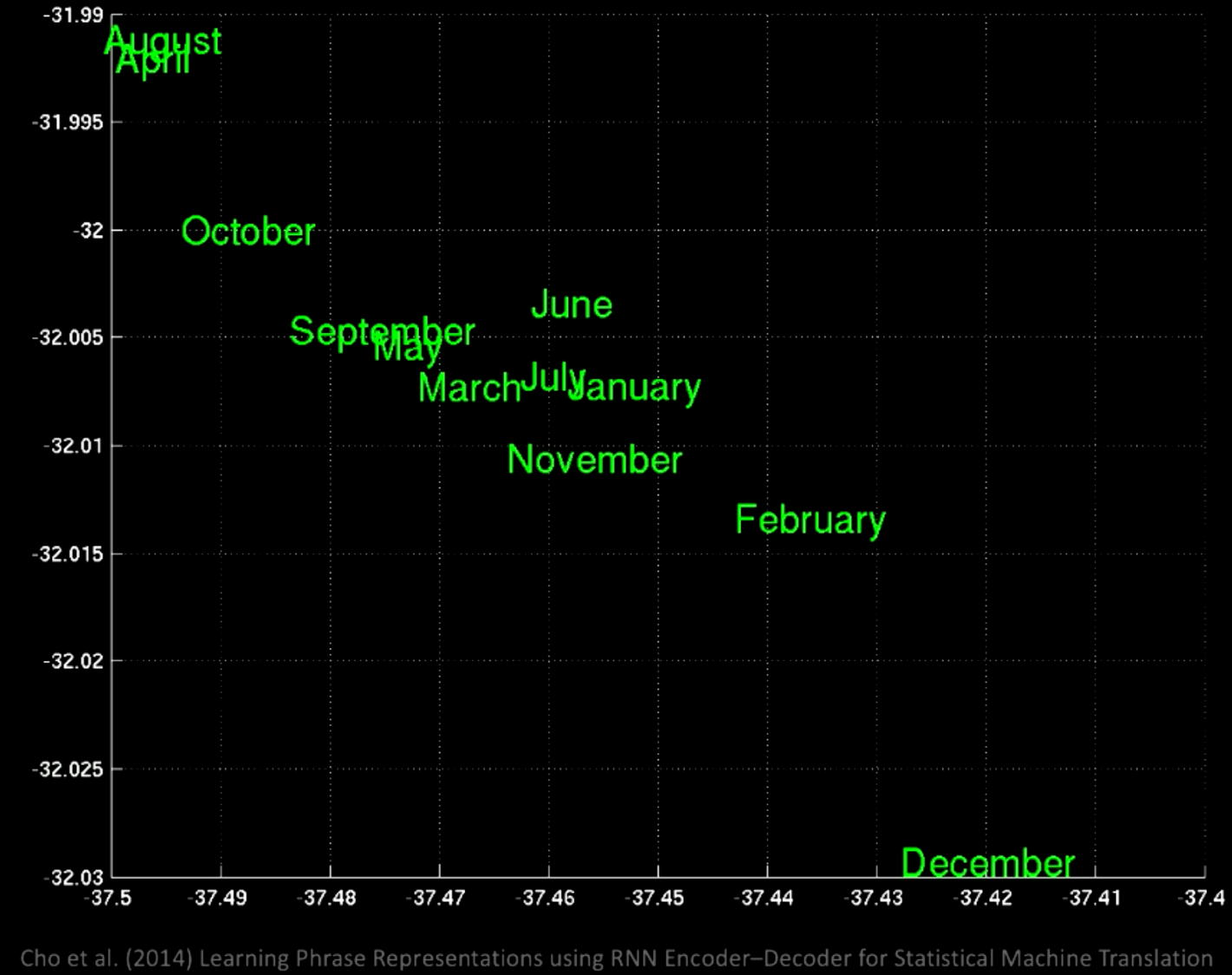
Figure 12: Zooming in Word Groups

If you focus on a different region, you get phrases like “a few days ago “ “the next few months” etc.

Figure 13: Word Groups in another Region

From these examples, we see that different locations will have some specific common meanings.

Figure 14 showcases how how by training this kind of network will pick up on some semantics features. For exmaple in this case you can see there is a vector connecting man to woman and another between king and queen, which means woman minus man is going to be equal to queen minus king. You will get the same distance in this embeddings space applied to cases like male-female. Another example will be walking to walked and swimming to swam. You can always apply this kind of specific linear transofmation going from one word to another or from country to capital.

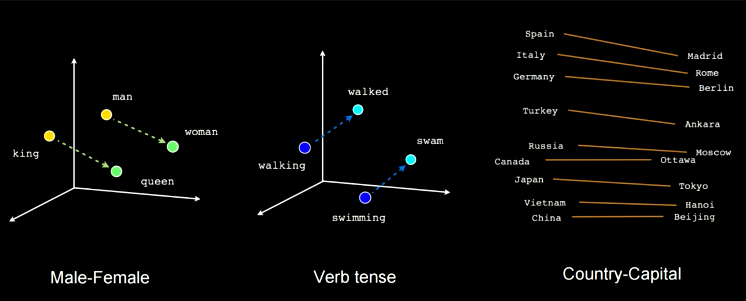
Figure 14: Semantics Features Picked during Training

The fourth and final case is sequence to sequence. In this network, as you start feeding in input the network starts generating outputs. An example of this type of architecture is T9, if you remember using a Nokia phone, you would get text suggestions as you were typing. Another example is speech to captions. One cool example is this RNN-writer. When you start typing “the rings of Saturn glittered while”, it suggests the following “two men looked at each other”. This network was trained on some sci-fi novels so that you can just type something and let it make suggestions to help you write a book. One more example is shown in Figure 16. You input the top prompt and then this network will try to complete the rest.

Figure 15: Seq to Seq

Figure 16: Text Auto-Completion Model of Seq to Seq Model

Back Propagation through time

Model architecture

In order to train an RNN, backpropagation through time (BPTT) must be used. The model architecture of RNN is given in the figure below. The left design uses loop representation while the right figure unfolds the loop into a row over time.

Figure 17: Back Propagation through time

Hidden representations are stated as

The first equation indicates a non-linear function applied on a rotation of a stack version of input where the previous configuration of the hidden layer is appended. At the beginning, $h[0]$ is set 0. To simplify the equation, $W_h$ can be written as two separate matrices, $\left[ W_{hx}\ W_{hh}\right]$, thus sometimes the transformation can be stated as

which corresponds to the stack representation of the input.

$y[t]$ is calculated at the final rotation and then we can use the chain rule to backpropagate the error to the previous time step.

Batch-Ification in Language Modeling

When dealing with a sequence of symbols, we can batchify the text into different sizes. For example, when dealing with sequences shown in the following figure, batch-ification can be applied first, where the time domain is preserved vertically. In this case, the batch size is set to 4.

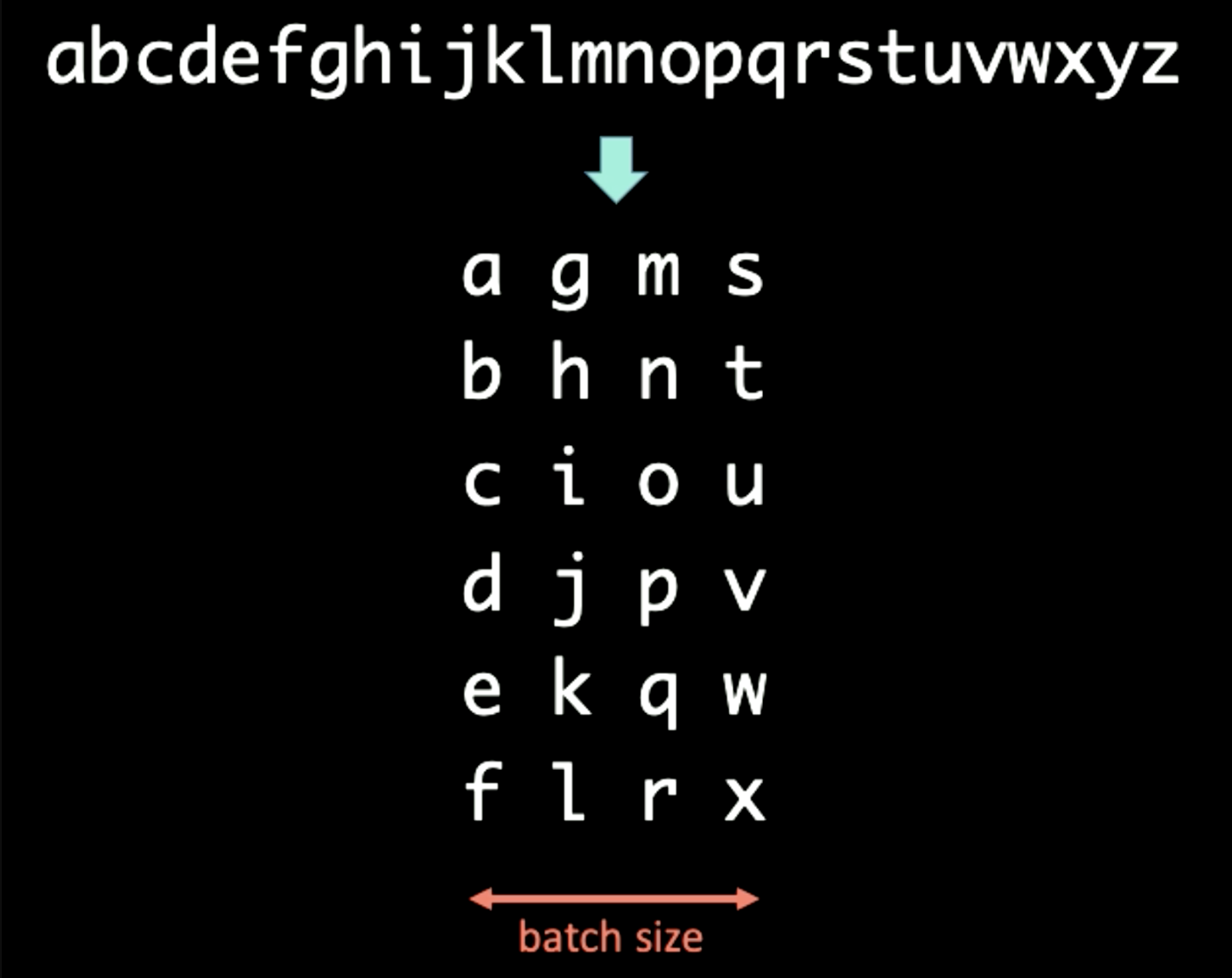
Figure 18: Batch-Ification

If BPTT period $T$ is set to 3, the first input $x[1:T]$ and output $y[1:T]$ for RNN is determined as

When performing RNN on the first batch, firstly, we feed $x[1] = [a\ g\ m\ s]$ into RNN and force the output to be $y[1] = [b\ h\ n\ t]$. The hidden representation $h[1]$ will be sent forward into next time step to help the RNN predict $y[2]$ from $x[2]$. After sending $h[T-1]$ to the final set of $x[T]$ and $y[T]$, we cut gradient propagation process for both $h[T]$ and $h[0]$ so that gradients will not propagate infinitely(.detach() in Pytorch). The whole process is shown in figure below.

Figure 19: Batch-Ification

Vanishing and Exploding Gradient

Problem

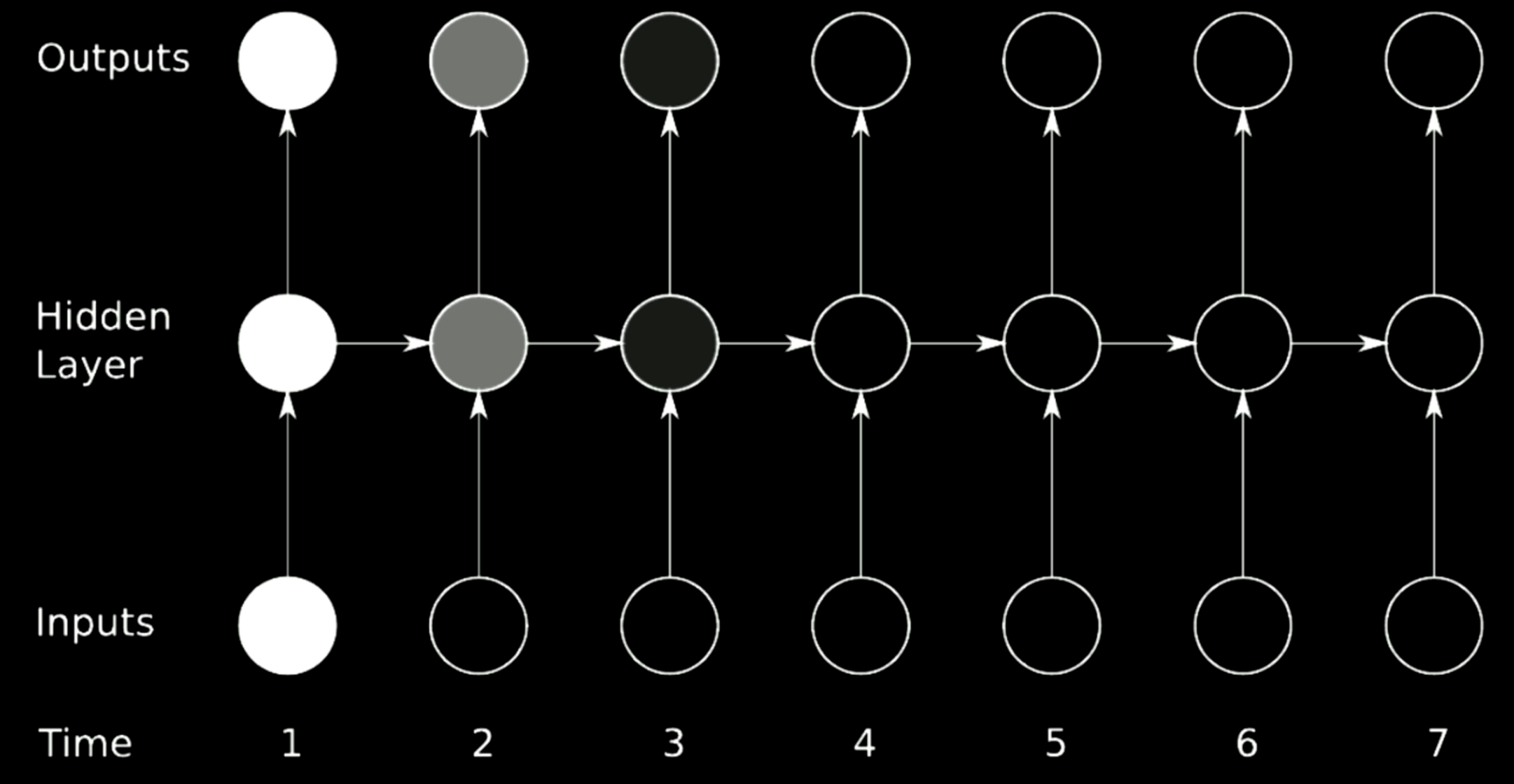
Figure 20: Vanishing Problem

The figure above is a typical RNN architecture. In order to perform rotation over previous steps in RNN, we use matrices, which can be regarded as horizontal arrows in the model above. Since the matrices can change the size of outputs, if the determinant we select is larger than 1, the gradient will inflate over time and cause gradient explosion. Relatively speaking, if the eigenvalue we select is small across 0, the propagation process will shrink gradients and leads to the gradient vanishing.

In typical RNNs, gradients will be propagated through all the possible arrows, which provides the gradients a large chance to vanish or explode. For example, the gradient at time 1 is large, which is indicated by the bright color. When it goes through one rotation, the gradient shrinks a lot and at time 3, it gets killed.

Solution

An ideal to prevent gradients from exploding or vanishing is to skip connections. To fulfill this, multiply networks can be used.

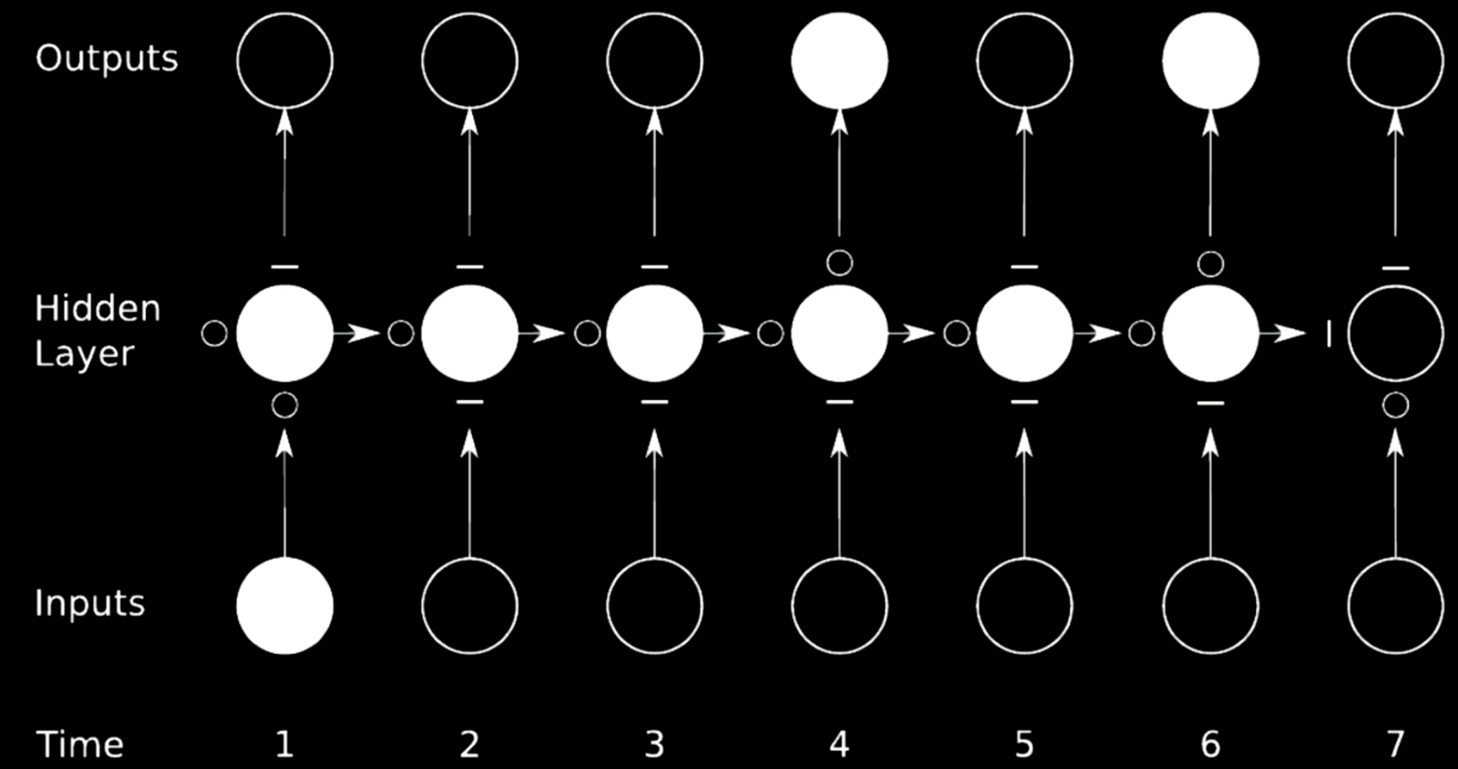
Figure 21: Skip Connection

In the case above, we split the original network into 4 networks. Take the first network for instance. It takes in a value from input at time 1 and sends the output to the first intermediate state in the hidden layer. The state has 3 other networks where the $\circ$s allows the gradients to pass while the $-$s blocks propagation. Such a technique is called gated recurrent network.

LSTM is one prevalent gated RNN and is introduced in detail in the following sections.

Long Short-Term Memory

Model Architecture

Below are equations expressing an LSTM. The input gate is highlighted by yellow boxes, which will be an affine transformation. This input transformation will be multiplying $c[t]$, which is our candidate gate.

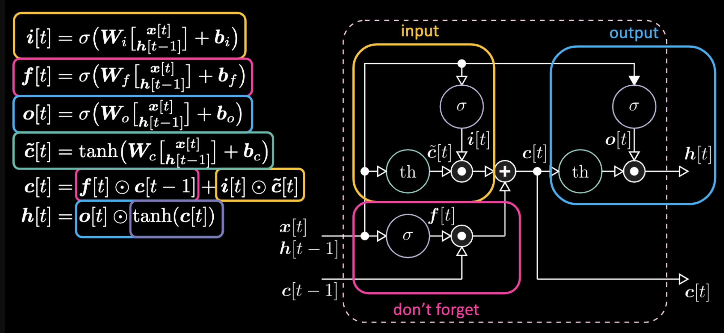
Figure 22: LSTM Architecture

Don’t forget gate is multiplying the previous value of cell memory $c[t-1]$. Total cell value $c[t]$ is don’t forget gate plus input gate. Final hidden representation is element-wise multiplication between output gate $o[t]$ and hyperbolic tangent version of the cell $c[t]$, such that things are bounded. Finally, candidate gate $\tilde{c}[t]$ is simply a recurrent net. So we have a $o[t]$ to modulate the output, a $f[t]$ to modulate the don’t forget gate, and a $i[t]$ to modulate the input gate. All these interactions between memory and gates are multiplicative interactions. $i[t]$, $f[t]$ and $o[t]$ are all sigmoids, going from zero to one. Hence, when multiplying by zero, you have a closed gate. When multiplying by one, you have an open gate.

How do we turn off the output? Let’s say we have a purple internal representation $th$ and put a zero in the output gate. Then the output will be zero multiplied by something, and we get a zero. If we put a one in the output gate, we will get the same value as the purple representation.

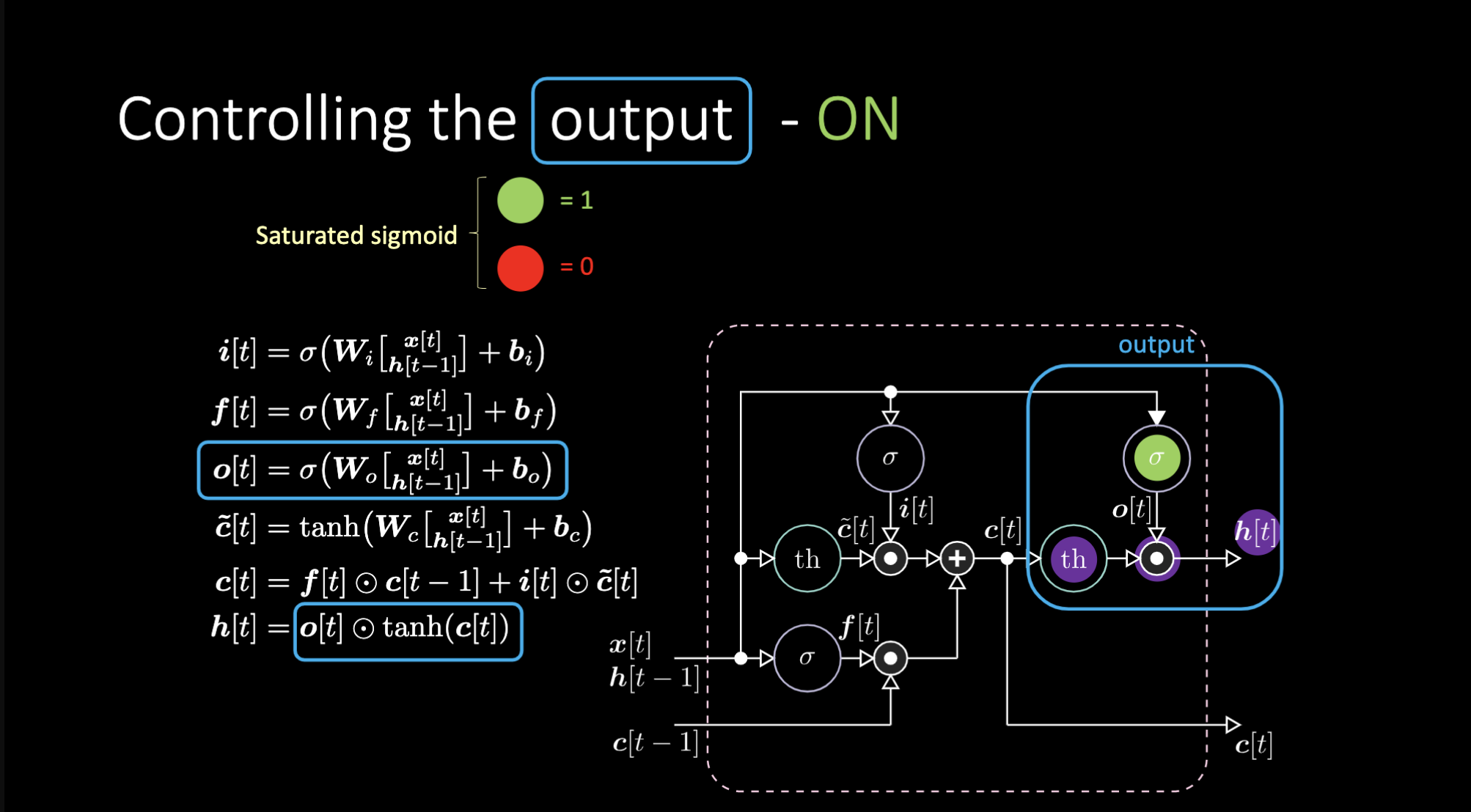
Figure 23: LSTM Architecture - Output On

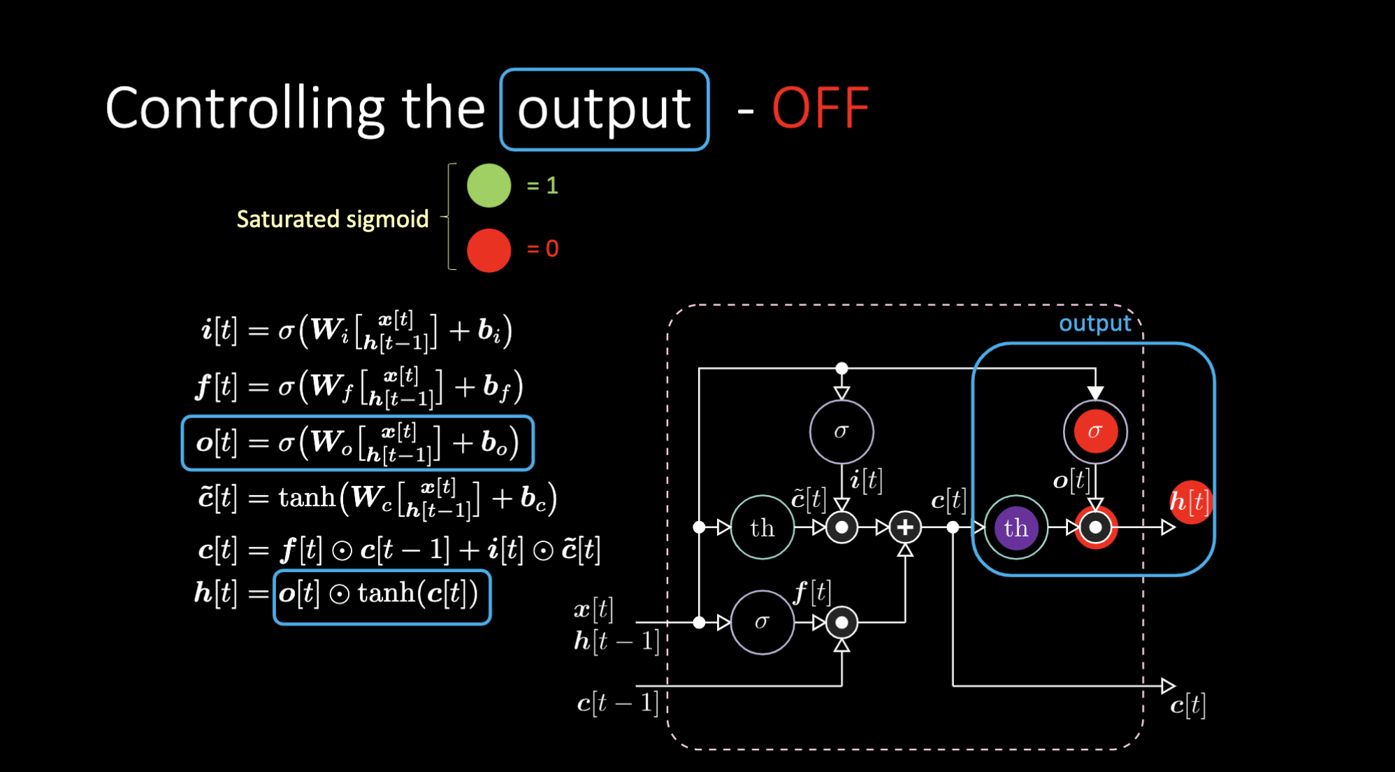
Figure 24: LSTM Architecture - Output Off

Similarly, we can control the memory. For example, we can reset it by having $f[t]$ and $i[t]$ to be zeros. After multiplication and summation, we have a zero inside the memory. Otherwise, we can keep the memory, by still zeroing out the internal representation $th$ but keep a one in $f[t]$. Hence, the sum gets $c[t-1]$ and keeps sending it out. Finally, we can write such that we can get a one in the input gate, the multiplication gets purple, then set a zero in the don’t forget gate so it actually forget.

Figure 25: Visualization of the Memory Cell

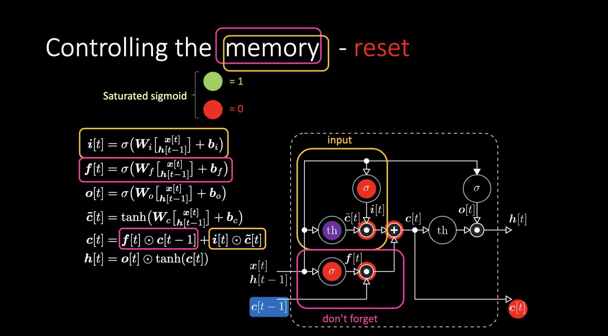
Figure 26: LSTM Architecture - Reset Memory

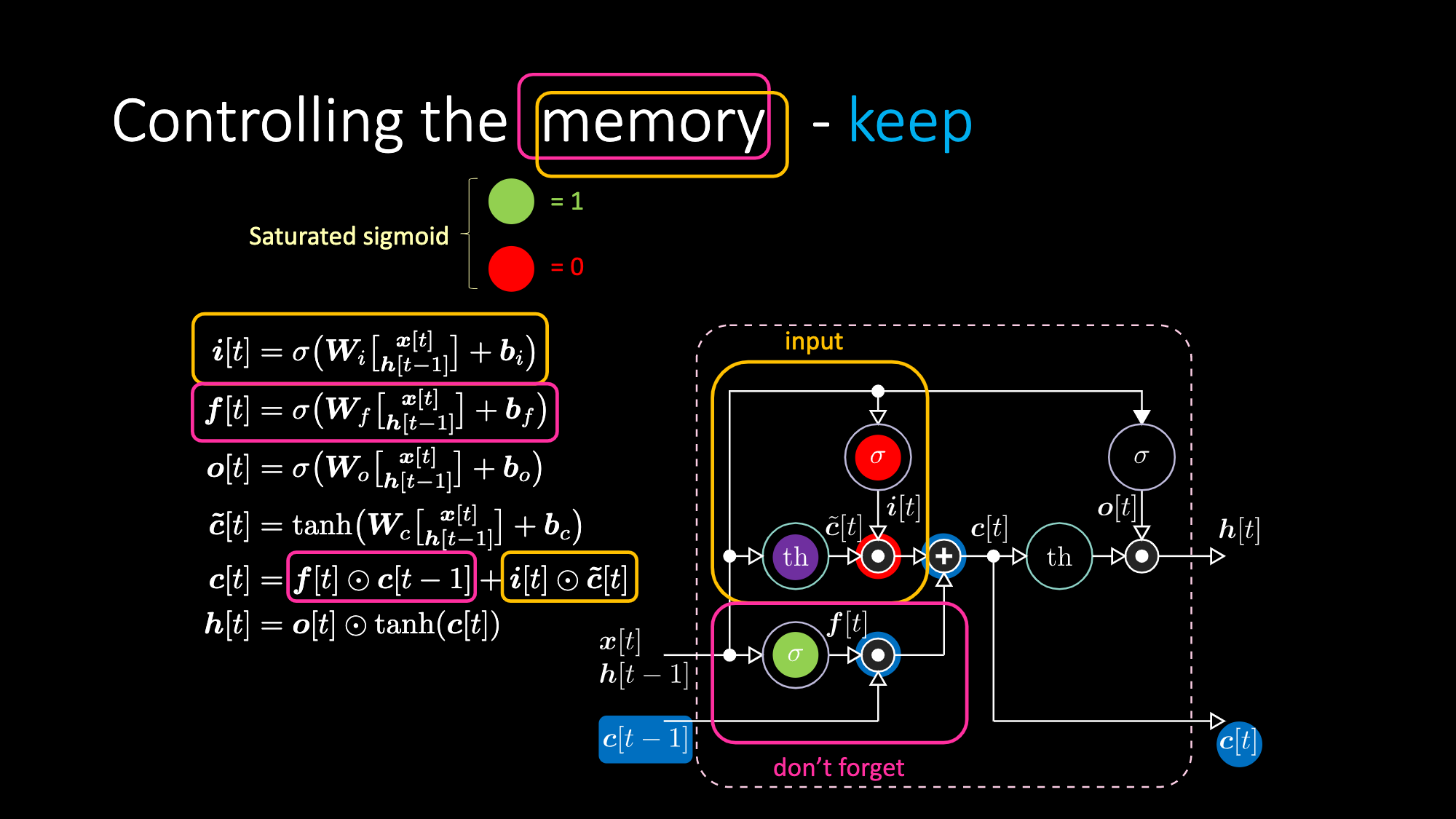
Figure 27: LSTM Architecture - Keep Memory

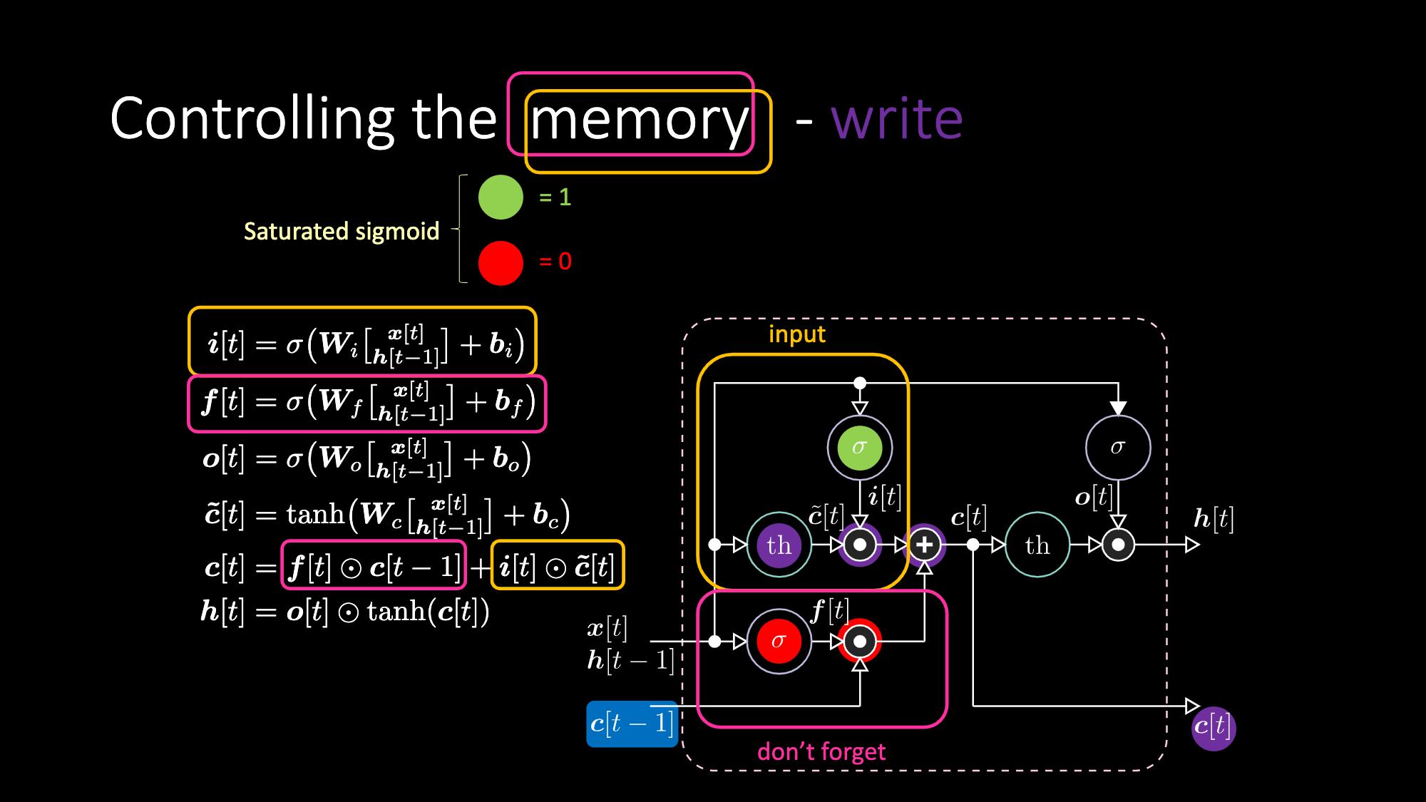
Figure 28: LSTM Architecture - Write Memory

Notebook Examples

Sequence Classification

The goal is to classify sequences. Elements and targets are represented locally (input vectors with only one non-zero bit). The sequence begins with an B, ends with a E (the “trigger symbol”), and otherwise consists of randomly chosen symbols from the set {a, b, c, d} except for two elements at positions $t_1$ and $t_2$ that are either X or Y. For the DifficultyLevel.HARD case, the sequence length is randomly chosen between 100 and 110, $t_1$ is randomly chosen between 10 and 20, and $t_2$ is randomly chosen between 50 and 60. There are 4 sequence classes Q, R, S, and U, which depend on the temporal order of X and Y. The rules are: X, X -> Q; X, Y -> R; Y, X -> S; Y, Y -> U.

1). Dataset Exploration

The return type from a data generator is a tuple with length 2. The first item in the tuple is the batch of sequences with shape $(32, 9, 8)$. This is the data going to be fed into the network. There are eight different symbols in each row (X, Y, a, b, c, d, B, E). Each row is a one-hot vector. A sequence of rows represents a sequence of symbols. The first all-zero row is padding. We use padding when the length of the sequence is shorter than the maximum length in the batch. The second item in the tuple is the corresponding batch of class labels with shape $(32, 4)$, since we have 4 classes (Q, R, S, and U). The first sequence is: BbXcXcbE. Then its decoded class label is $[1, 0, 0, 0]$, corresponding to Q.

Figure 29: Input Vector Example

2). Defining the Model and Training

Let’s create a simple recurrent network, an LSTM, and train for 10 epochs. In the training loop, we should always look for five steps:

• Perform the forward pass of the model
• Compute the loss
• Zero the gradient cache
• Backpropagate to compute the partial derivative of loss with regard to parameters
• Step in the opposite direction of the gradient

Figure 30: Simple RNN *vs.* LSTM - 10 Epochs

With an easy level of difficulty, RNN gets 50% accuracy while LSTM gets 100% after 10 epochs. But LSTM has four times more weights than RNN and has two hidden layers, so it is not a fair comparison. After 100 epochs, RNN also gets 100% accuracy, taking longer to train than the LSTM.

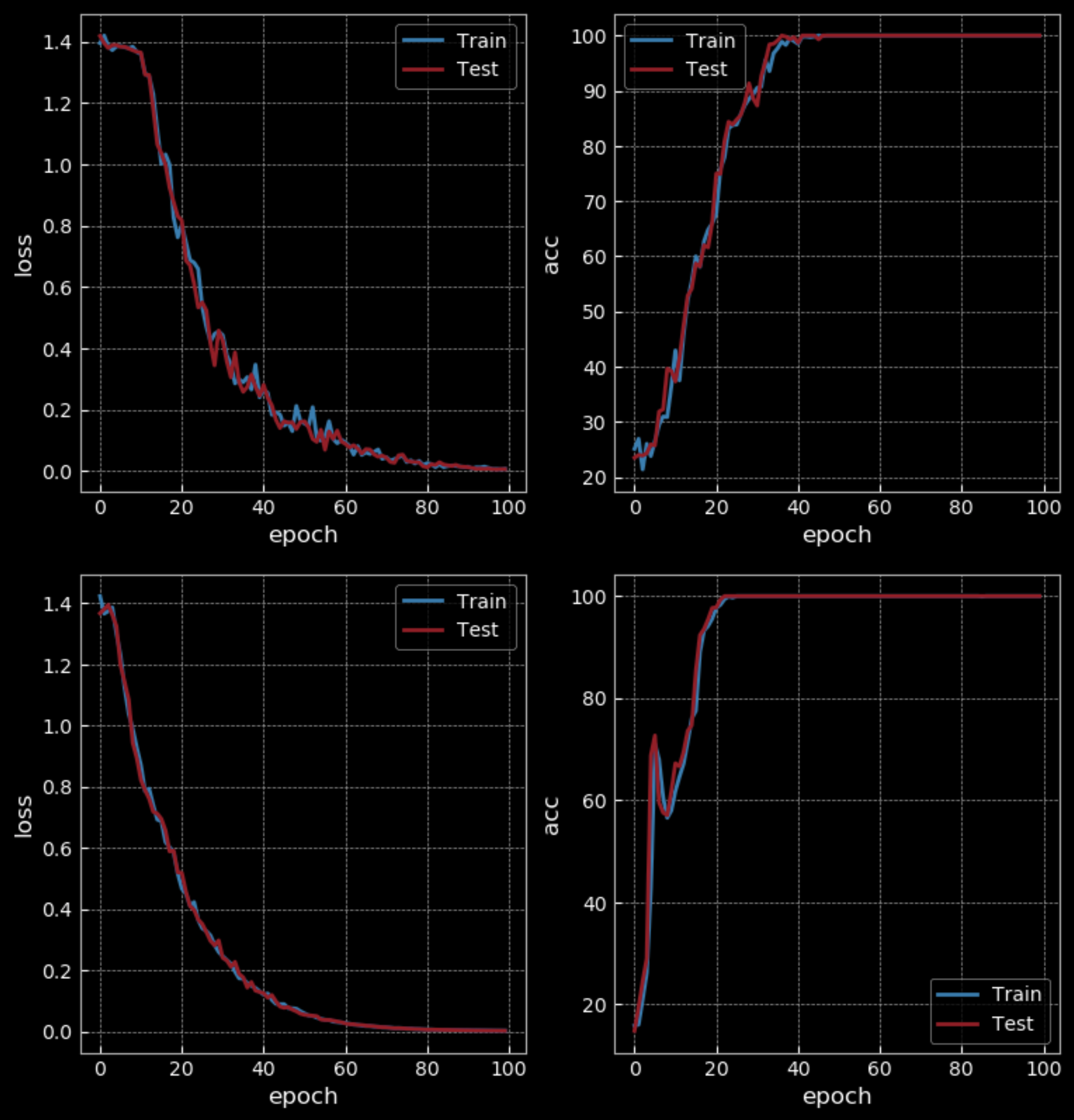
Figure 31: Simple RNN *vs.* LSTM - 100 Epochs

If we increase the difficulty of the training part (using longer sequences), we will see the RNN fails while LSTM continues to work.

Figure 32: Visualization of Hidden State Value

The above visualization is drawing the value of hidden state over time in LSTM. We will send the inputs through a hyperbolic tangent, such that if the input is below $-2.5$, it will be mapped to $-1$, and if it is above $2.5$, it will be mapped to $1$. So in this case, we can see the specific hidden layer picked on X (fifth row in the picture) and then it became red until we got the other X. So, the fifth hidden unit of the cell is triggered by observing the X and goes quiet after seeing the other X. This allows us to recognize the class of sequence.

Signal Echoing

Echoing signal n steps is an example of synchronized many-to-many task. For instance, the 1st input sequence is "1 1 0 0 1 0 1 1 0 0 0 0 0 0 0 0 1 1 1 1 ...", and the 1st target sequence is "0 0 0 1 1 0 0 1 0 1 1 0 0 0 0 0 0 0 0 1 ...". In this case, the output is three steps after. So we need a short-time working memory to keep the information. Whereas in the language model, it says something that hasn’t already been said.

Before we send the whole sequence to the network and force the final target to be something, we need to cut the long sequence into little chunks. While feeding a new chunk, we need to keep track of the hidden state and send it as input to the internal state when adding the next new chunk. In LSTM, you can keep the memory for a long time as long as you have enough capacity. In RNN, after you reach a certain length, it starts to forget about what happened in the past.