Computing gradients for NN modules and Practical tricks for Back Propagation

A concrete example of backpropagation and intro to basic neural network modules

Example

We next consider a concrete example of backpropagation assisted by a visual graph. The arbitrary function $G(w)$ is input into the cost function $C$, which can be represented as a graph. Through the manipulation of multiplying the Jacobian matrices, we can transform this graph into the graph that will compute the gradients going backwards. (Note that PyTorch and TensorFlow do this automatically for the user, i.e. the forward graph is automatically “reversed” to create the derivative graph that backpropagates the gradient.)

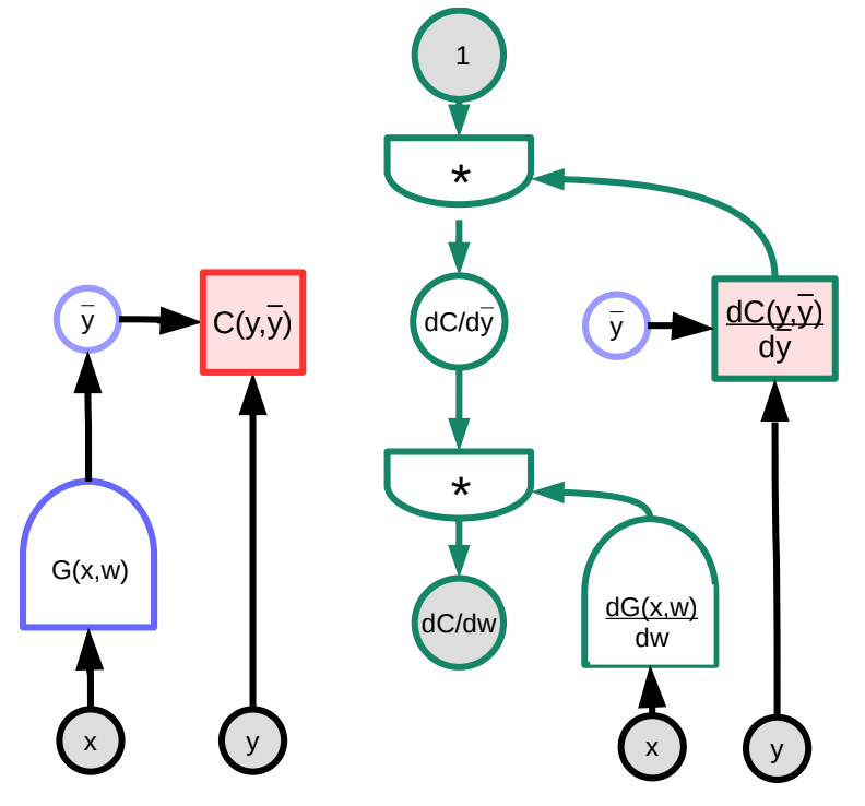
In this example, the green graph on the right represents the gradient graph. Following the graph from the topmost node, it follows that

In terms of dimensions, $\frac{\partial C(y,\bar{y})}{\partial w}$ is a row vector of size $1\times N$ where $N$ is the number of components of $w$; $\frac{\partial C(y,\bar{y})}{\partial \bar{y}}$ is a row vector of size $1\times M$, where $M$ is the dimension of the output; $\frac{\partial \bar{y}}{\partial w}=\frac{\partial G(x,w)}{\partial w}$ is a matrix of size $M\times N$, where $M$ is the number of outputs of $G$ and $N$ is the dimension of $w$.

Note that complications might arise when the architecture of the graph is not fixed, but is data-dependent. For example, we could choose neural net module depending on the length of input vector. Though this is possible, it becomes increasingly difficult to manage this variation when the number of loops exceeds a reasonable amount.

Basic neural net modules

There exist different types of pre-built modules besides the familiar Linear and ReLU modules. These are useful because they are uniquely optimized to perform their respective functions (as opposed to being built by a combination of other, elementary modules).

• Linear: $Y=W\cdot X$

  \[\begin{aligned} \frac{dC}{dX} &= W^\top \cdot \frac{dC}{dY} \\ \frac{dC}{dW} &= \frac{dC}{dY} \cdot X^\top \end{aligned}\]

• ReLU: $y=(x)^+$

  \[\frac{dC}{dX} = \begin{cases} 0 & x<0\\ \frac{dC}{dY} & \text{otherwise} \end{cases}\]

• Duplicate: $Y_1=X$, $Y_2=X$

  • Akin to a “Y - splitter” where both outputs are equal to the input.

  • When backpropagating, the gradients get summed

  • Can be split into $n$ branches similarly

    \[\frac{dC}{dX}=\frac{dC}{dY_1}+\frac{dC}{dY_2}\]

• Add: $Y=X_1+X_2$

  • With two variables being summed, when one is perturbed, the output will be perturbed by the same quantity, i.e.

    \[\frac{dC}{dX_1}=\frac{dC}{dY}\cdot1 \quad \text{and}\quad \frac{dC}{dX_2}=\frac{dC}{dY}\cdot1\]

• Max: $Y=\max(X_1,X_2)$

  • Since this function can also be represented as
  \[Y=\max(X_1,X_2)=\begin{cases} X_1 & X_1 > X_2 \\ X_2 & \text{else} \end{cases} \Rightarrow \frac{dY}{dX_1}=\begin{cases} 1 & X_1 > X_2 \\ 0 & \text{else} \end{cases}\]

  • Therefore, by the chain rule,

    \[\frac{dC}{dX_1}=\begin{cases} \frac{dC}{dY}\cdot1 & X_1 > X_2 \\ 0 & \text{else} \end{cases}\]

LogSoftMax vs. SoftMax

SoftMax, which is also a PyTorch module, is a convenient way of transforming a group of numbers into a group of positive numbers between $0$ and $1$ that sum to one. These numbers can be interpreted as a probability distribution. As a result, it is commonly used in classification problems. $y_i$ in the equation below is a vector of probabilities for all the categories.

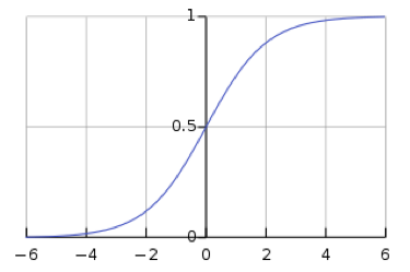
However, the use of softmax leaves the network susceptible to vanishing gradients. Vanishing gradient is a problem, as it prevents weights downstream from being modified by the neural network, which may completely stop the neural network from further training. The logistic sigmoid function, which is the softmax function for one value, shows that when $s$ is large, $h(s)$ is $1$, and when s is small, $h(s)$ is $0$. Because the sigmoid function is flat at $h(s) = 0$ and $h(s) = 1$, the gradient is $0$, which results in a vanishing gradient.

Mathematicians came up with the idea of logsoftmax in order to solve for the issue of the vanishing gradient created by softmax. LogSoftMax is another basic module in PyTorch. As can be seen in the equation below, LogSoftMax is a combination of softmax and log.

The equation below demonstrates another way to look at the same equation. The figure below shows the $\log(1 + \exp(s))$ part of the function. When $s$ is very small, the value is $0$, and when $s$ is very large, the value is $s$. As a result it doesn’t saturate, and the vanishing gradient problem is avoided.

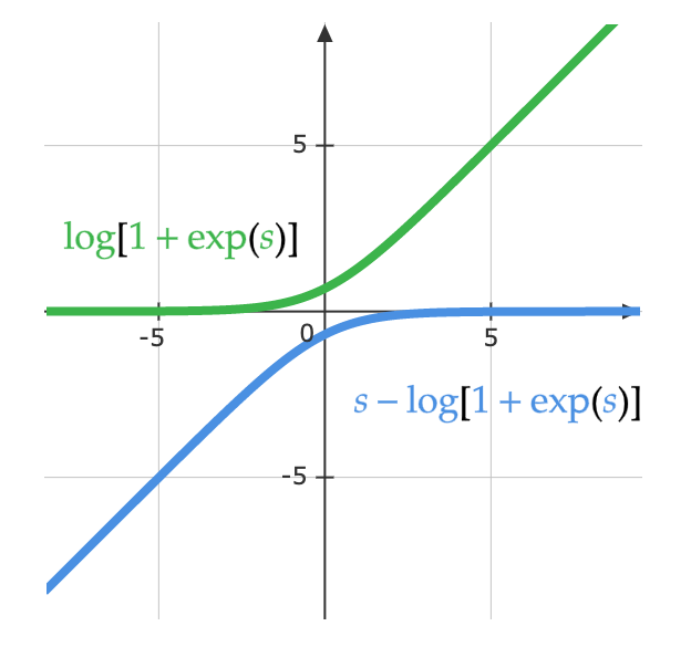
Practical tricks for backpropagation

Use ReLU as the non-linear activation function

ReLU works best for networks with many layers, which has caused alternatives like the sigmoid function and hyperbolic tangent $\tanh(\cdot)$ function to fall out of favour. The reason ReLU works best is likely due to its single kink which makes it scale equivariant.

Use cross-entropy loss as the objective function for classification problems

Log softmax, which we discussed earlier in the lecture, is a special case of cross-entropy loss. In PyTorch, be sure to provide the cross-entropy loss function with log softmax as input (as opposed to normal softmax).

Use stochastic gradient descent on minibatches during training

As discussed previously, minibatches let you train more efficiently because there is redundancy in the data; you shouldn’t need to make a prediction and calculate the loss on every single observation at every single step to estimate the gradient.

Shuffle the order of the training examples when using stochastic gradient descent

Order matters. If the model sees only examples from a single class during each training step, then it will learn to predict that class without learning why it ought to be predicting that class. For example, if you were trying to classify digits from the MNIST dataset and the data was unshuffled, the bias parameters in the last layer would simply always predict zero, then adapt to always predict one, then two, etc. Ideally, you should have samples from every class in every minibatch.

However, there’s ongoing debate over whether you need to change the order of the samples in every pass (epoch).

Normalize the inputs to have zero mean and unit variance

Before training, it’s useful to normalize each input feature so that it has a mean of zero and a standard deviation of one. When using RGB image data, it is common to take mean and standard deviation of each channel individually and normalize the image channel-wise. For example, take the mean $m_b$ and standard deviation $\sigma_b$ of all the blue values in the dataset, then normalize the blue values for each individual image as

where $\epsilon$ is an arbitrarily small number that we use to avoid division by zero. Repeat the same for green and red channels. This is necessary to get a meaningful signal out of images taken in different lighting; for example, day lit pictures have a lot of red while underwater pictures have almost none.

Use a schedule to decrease the learning rate

The learning rate should fall as training goes on. In practice, most advanced models are trained by using algorithms like Adam which adapt the learning rate instead of simple SGD with a constant learning rate.

Use L1 and/or L2 regularization for weight decay

You can add a cost for large weights to the cost function. For example, using L2 regularization, we would define the loss $L$ and update the weights $w$ as follows:

To understand why this is called weight decay, note that we can rewrite the above formula to show that we multiply $w_i$ by a constant less than one during the update.

L1 regularization (Lasso) is similar, except that we use $\sum_i \vert w_i\vert$ instead of $\Vert w \Vert^2$.

Essentially, regularization tries to tell the system to minimize the cost function with the shortest weight vector possible. With L1 regularization, weights that are not useful are shrunk to $0$.

Weight initialisation

The weights need to be initialised at random, however, they shouldn’t be too large or too small such that output is roughly of the same variance as that of input. There are various weight initialisation tricks built into PyTorch. One of the tricks that works well for deep models is Kaiming initialisation where the standard deviation of the weights is inversely proportional to square root of number of inputs.

Use dropout

Dropout is another form of regularization. It can be thought of as another layer of the neural net: it takes inputs, randomly sets $n/2$ of the inputs to zero, and returns the result as output. This forces the system to take information from all input units rather than becoming overly reliant on a small number of input units thus distributing the information across all of the units in a layer. This method was initially proposed by Hinton et al (2012).

For more tricks, see LeCun et al 1998.

Finally, note that backpropagation doesn’t just work for stacked models; it can work for any directed acyclic graph (DAG) as long as there is a partial order on the modules.