Deep Learning for Structured Prediction

Structured prediction

It is the problem of predicting variable y for a given input x which is mutually dependent and constrained rather than scalar discrete or real values. The output variable does not belong to a single category but can have exponential or infinite possible values. For example, in case of speech/handwriting recognition or natural language translation, the output needs to be grammatically correct and it is not possible to limit the number of output possibilities. The task of the model is to capture the sequential, spatial, or combinatorial structure in the problem domain.

Early works on structured prediction

This vector is fed to a TDNN which gives a feature vector which in case of model systems can be compared to softmax that represents a category. One problem that arises in the case of recognizing the word that was pronounced is different people can pronounce the same word in different ways and speed. To solve this Dynamic Time Warping is used.

The idea is to provide the system with a set of pre-recorded templates that correspond to sequence or feature vectors that were recorded by someone. The neural network is trained at the same time as the template so that the system learns to recognize the word for different pronunciations. The latent variable allows us to time-warp the feature vector so as to match the length of the templates.

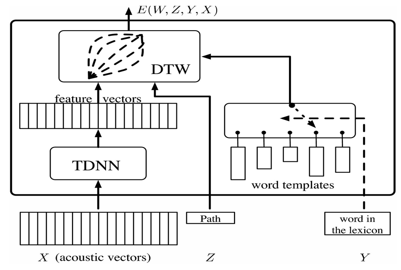
Figure 1.

This can be visualized as a matrix by arranging the feature vectors from TDNN horizontally and the word templates vertically. Each entry in the matrix corresponds to the distance between the feature vector. This can be visualized as a graph problem where the aim is to start from the bottom left-hand corner and reach the top right corner by traversing the path that minimizes the distance.

To train this latent variable model we need to make the energy for the correct answers as small as possible and larger for every incorrect answer. To do this we use an objective function that takes in templates for wrong words and pushes them away from the current sequence of features and backpropagates the gradients.

Energy based factor graphs

The idea behind energy-based factor graphs is to build an energy-based model in which the energy is sum of partial energy terms or when the probability is a product of factors. The benefit of these models is that efficient inference algorithms can be employed.

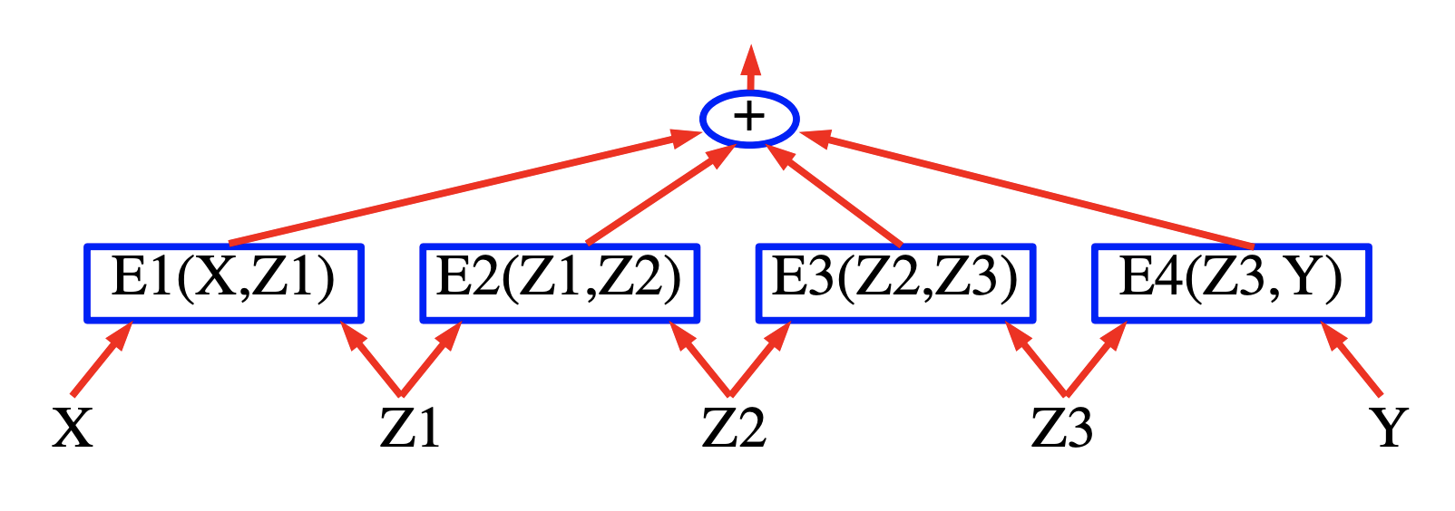
Figure 2.

Sequence labelling

The model takes an input speech signal X and output the labels Y such that the output labels minimize the total energy term.

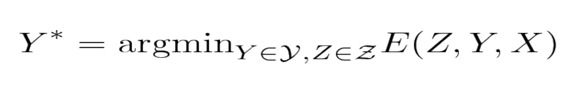
Figure 3.

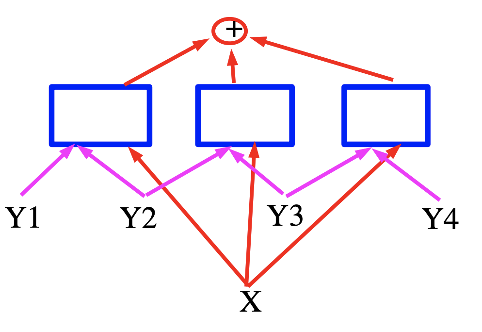
Figure 4.

In this case, the energy is a sum of three terms represented by blue squares which are neural networks that produce feature vectors for the input variables. In the case of speech recognition X can be thought of as a speech signal and the squares implement the grammatical constraints and Y represent the generated output labels.

Efficient inference for energy-based factor graphs

A Tutorial on Energy-Based Learning (Yann LeCun, Sumit Chopra, Raia Hadsell, Marc’Aurelio Ranzato, and Fu Jie Huang 2006):

Learning and inference with Energy-Based Models involves a minimization of the energy over the set of answers $\mathcal{Y}$ and latent variables $\mathcal{Z}$. When the cardinality of $\mathcal{Y}\times \mathcal{Z}$ is large, this minimization can become intractable. One approach to the problem is to exploit the structure of the energy function in order to perform the minimization efficiently. One case where the structure can be exploited occurs when the energy can be expressed as a sum of individual functions (called factors) that each depend on different subsets of the variables in Y and Z. These dependencies are best expressed in the form of a factor graph. Factor graphs are a general form of graphical models, or belief networks.

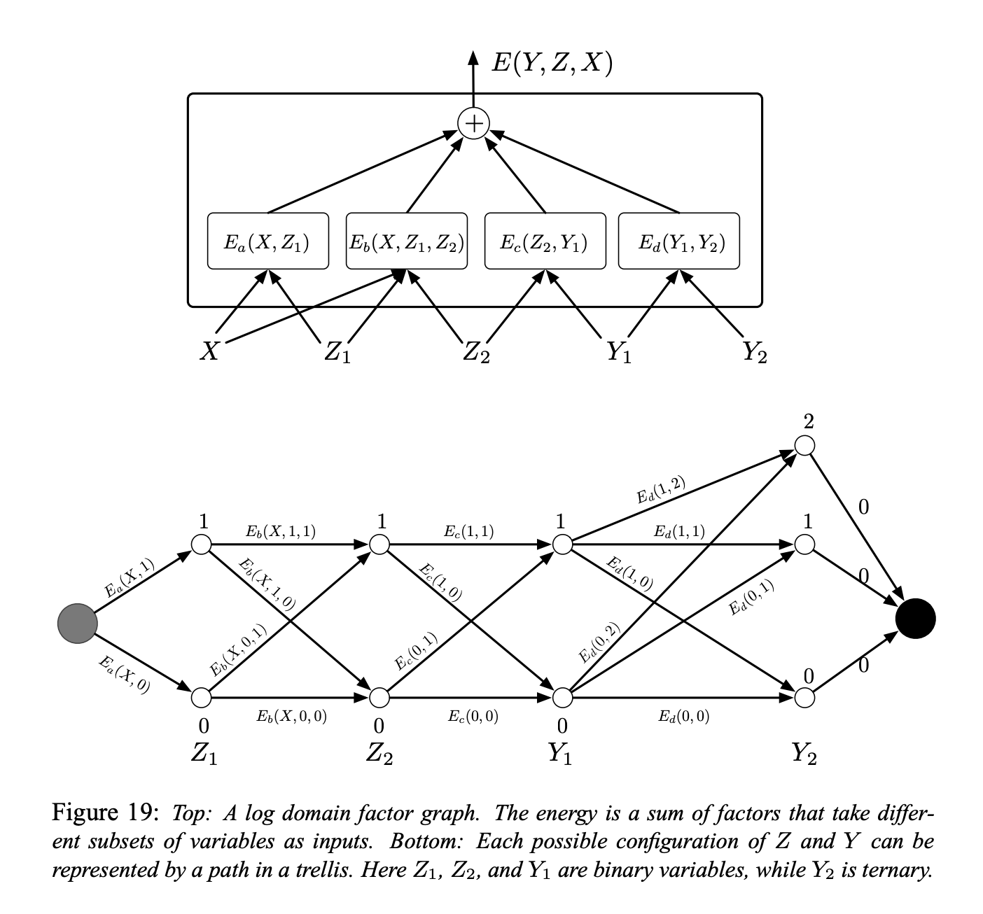
Figure 5.

A simple example of a factor graph is shown in Figure 19 (top). The energy function is the sum of four factors:

where $Y = [Y_1, Y_2]$ are the output variables and $Z = [Z_1, Z_2]$ are the latent variables. Each factor can be seen as representing soft constraints between the values of its input variables. The inference problem consists in finding:

Let’s assume that $Z_1$, $Z_2$, and $Y_1$ are discrete binary variables, and $Y_2$ is a ternary variable. The cardinality of the domain of $X$ is immaterial since X is always observed. The number of possible configurations of $Z$ and $Y$ given X is $2 \times 2 \times 2 \times 3 = 24$. A naive minimization algorithm through exhaustive search would evaluate the entire energy function 24 times (96 single factor evaluations).

However, we notice that for a given $X$, $E_a$ only has two possible input configurations: $Z_1 = 0$ and $Z_1 = 1$. Similarly, $E_b$ and $E_c$ only have 4 possible input configurations, and $E_d$ has 6. Hence, there is no need for more than $2 + 4 + 4 + 6 = 16$ single factor evaluations.

Hence, we can pre compute the 16 factor values, and put them on the arcs in a trellis as shown in Figure 5 (bottom).

The nodes in each column represent the possible values of a single variable. Each edge is weighted by the output energy of the factor for the corresponding values of its input variables. With this representation, a single path from the start node to the end node represents one possible configuration of all the variables. The sum of the weights along a path is equal to the total energy for the corresponding configuration. Therefore, the inference problem can be reduced to searching for the shortest path in this graph. This can be performed using a dynamic programming method such as the Viterbi algorithm, or the A* algorithm. The cost is proportional to the number of edges (16), which is exponentially smaller than the number of paths in general.

To compute $E(Y, X) = \min_{z\in Z} E(Y, z, X)$, we follow the same procedure, but we restrict the graph to the subset of arcs that are compatible with the prescribed value of $Y$.

The above procedure is sometimes called the min-sum algorithm, and it is the log domain version of the traditional max-product for graphical models. The procedure can easily be generalized to factor graphs where the factors take more than two variables as inputs, and to factor graphs that have a tree structure instead of a chain structure.

However, it only applies to factor graphs that are bipartite trees (with no loops). When loops are present in the graph, the min-sum algorithm may give an approximate solution when iterated, or may not converge at all. In this case, a descent algorithm such as simulated annealing could be used.

Simple energy-based factor graphs with “shallow” factors

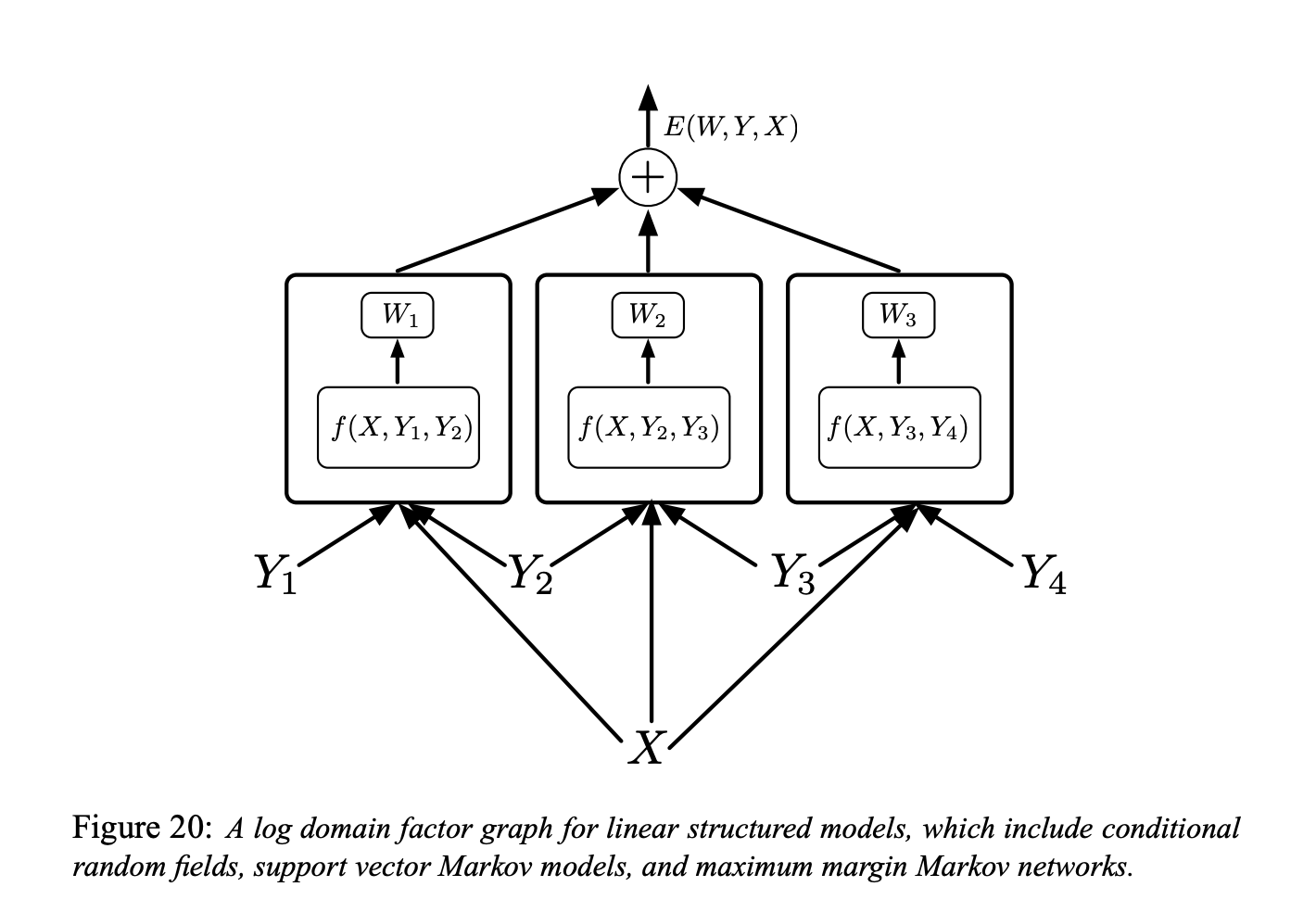
Figure 6.

The factor graph shown in Figure 6 is a log domain factor graph for linear structured models (“simple energy-based factor graphs” we are talking about)

Each factor is a linear function of the trainable parameters. It depends on the input $X$ and on a pair of individual labels $(Y_m, Y_n)$. In general, each factor could depend on more than two individual labels, but we will limit the discussion to pairwise factors to simplify the notation:

Here $\mathcal{F}$ denotes the set of factors (the set of pairs of individual labels that have a direct inter-dependency), $W_{m n}$ is the parameter vector for factor $(m, n),$ and $f_{m n}\left(X, Y_{m}, Y_{n}\right)$ is a (fixed) feature vector. The global parameter vector $W$ is the concatenation of all the $W_{m n}.$

And then we can think about like what type of loss function. Here comes several different models.

Conditional Random Field

We can use the negative log-likelihood loss function to train a linear structured model.

This is the Conditional Random Field

The intuition is we want the energy of the correct answer to below and want the log of exponential for all the answers, including the good one, to be large.

Below is the formal definition for the negative log-likelihood loss function:

Max-margin Markov nets and latent SVM

We can also using the Hinge loss function for optimization.

The intuition behind is that we want the energy of the correct answer to be low, and then among all possible configurations of incorrect answers, we are going to look for the one that has the lowest energy among all the wrong or the bad ones. And then we are going to push up the energy of this one. We don’t need to push up the energy for the other bad answers because they are larger anyway.

This is the idea behind Max Margin Markov Nets and Latent SVM.

Structured perceptron model

We can train the linear structured model by using perceptron loss.

Collins [Collins, 2000, Collins, 2002] has advocated its use for linear structured models in the context of NLP:

where $Y^{* i}=\operatorname{argmin}_{y \in \mathcal{Y}} E\left(W, y, X^{i}\right)$ is the answer produced by the system.

Early trails on discriminative training for speech/handwritten recognition

Minimum Empirical Error Loss (Ljolje, and Rabiner 1990):

By training at sequence level, they do not tell the system this sound or that location. They give the system input sentence and transcription of it in term of words, and ask the system to figure it out by doing time warping. They did not use neural networks, and have other ways in turning speech signals into sound categories.

Graph Transformer Net

Here the problem is that we have a sequence of digits at the input and we do not know how to do segmentation. What we can do is build a graph in which each path is a way of breaking up the sequence of characters, and we are going to find out the path with lowest energy, basically is to find the shortest path. Here is a concrete example of how it works.

We have input image 34. Run this through segmenter, and get multiple alternative segmentations. These segmentation are ways to group these blobs of thing together. Each path in the segmentation graph corresponds to one particular way of grouping the blobs of ink.

Figure 7.

We run each through the same character recognition ConvNet, and get a list of 10 scores (Two here but essentially should be 10, representing 10 categories). For example, 1 [0.1] means the energy is 0.1 for category 1. So I get a graph here, and you can think of it as a weird form of tensor. It is a sparse tensor really. It is a tensor that says for each possible configuration of this variable, tell me the cost of the variable. It’s more like a distribution over tensors, or log distribution because we are talking about energies.

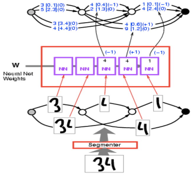
Figure 8.

Take this graph and then I want to compute the energy of the correct answer. I am telling you the correct answer is 34. Select within those paths and find out ones that say 34. There are two of them, one the energy 3.4 + 2.4 = 5.8, and the other 0.1 + 0.6 = 0.7. Pick the path with the lowest energy. Here we get the path with energy 0.7.

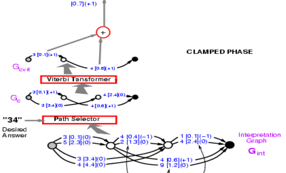
Figure 9.

So finding the path is like minimizing over the latent variable where latent variable is which path you pick. Conceptually, it is an energy model with latent variable as a path.

Now we have the energy of the correct path, 0.7. What we need to do now is backpropagate gradient through this entire structure, so that we can change the weight in ConvNet in such a way that final energy goes down. It looks daunting, but is entirely possible. Because this entire system is built out of element we already know about, neural net is regular and the Path Selector and Viterbi Transformer are basically switches that pick a particular edge or not.

So how do we backpropagate. Well, the point 0.7 is the sum of 0.1 and 0.6. So both point 0.1 and 0.6 will have gradient +1, which are indicated in the brackets. Then Viterbi Transformer just select one path among two. So just copy the gradient for the corresponding edge in the input graph and set the gradient for other paths that are not selected as zero. It’s exactly what’s happening in Max-Pooling or Mean-Pooling. The Path Selector is the same, it is just a system that selects the correct answer. Note that 3 [0.1] (0) in the graph should be 3 [0.1] (1) at this stage, and will come back to this later. Then you can backpropagate gradient through the neural net. That will make the energy of the correct answer small.

What’s important here is that this structure is dynamic in the sense that if I give you a new input, the number of instances of neural net will change with the number of segmentations, and graphs derived will also change. We need to backpropagate through this dynamical structure. This is the situation where things like PyTorch are really important.

This phase of backpropagation make the energy of correct answer small. And there’s going to be a second phase where we are going to make the energy of incorrect answer large. In this case, we just let the system pick whatever answer it wants. This is going to be a simplified form of discriminative training for structure prediction that use perceptual loss.

The first stages of phase two are exactly the same with the first phase. The Viterbi Transformer here just pick the best path with the lowest energy, we do not care whether this path is a correct path or not here. The energy you get here is going to be smaller or equal to the one you get from phase one, since the energy get here is the smallest among all possible paths.

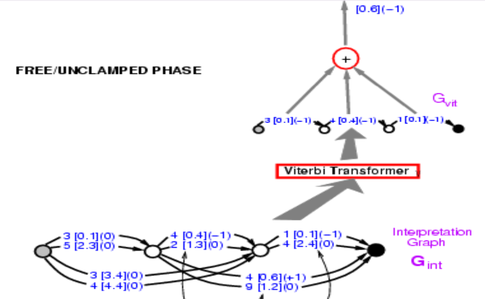
Figure 10.

Putting phase one and two together. The loss function should be energy1 - energy2. Before, we introduced how to backpropagate through the left part, and now we actually need to backpropagate through the entire structure. Whatever path on the left side will get +1, and whatever path in right hand side will get -1. So 3 [0.1] appeared in both path, thus should get gradient 0. If we do this, the system will eventually minimize the difference between the energy of the correct answer and the energy of the best answer whatever it is. The Loss function here is the perceptron loss.

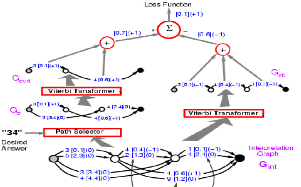
Figure 11.

Comprehension Questions and Answers

Question 1: Why is inference easy in the case of energy-based factor graphs?

Inference in the case of the energy-based model with latent variable involves the usage of exhaustive techniques such as gradient descent to minimize the energy however since the energy, in this case, is the sum of factors and techniques such as dynamic programming can be used instead.

Question 2: What if the latent variables in factor graphs are continuous variables? Can we still using min-sum algorithm?

We can’t since we can’t search for all possible combination for all factor values now. However, in this case, energies also gives us an advantage, because we can do independent optimizations. Like the combination of $Z_1$ and $Z_2$ only affects $E_b$ in Figure 19. We can do independent optimization and dynamic programming to do the inference.

Question 3: Are the NN boxes referring to separate ConvNets?

They are shared. They are multiple copies of the same ConvNet. It’s just a character recognition network.