Inference for latent variable Energy-Based Models (EBMs)

Training data and model definition

To understand why and how to use an Energy-Based Model (EBM), as well as relevant data format, let us consider training samples from an ellipse. Given function below

where $x \sim \mathcal{U}(0,1),\space \theta \sim \mathcal{U}(0,2\pi),\space \epsilon \sim \mathcal{N}[0, (\frac{1}{20})^2]$ and $\rho : \mathbb{R} \mapsto \mathbb{R}^2$ maps $x$ into \(\begin{bmatrix}\alpha x + \beta (1-x) \\ \beta x + \alpha (1-x) \end{bmatrix}\exp(2x)\).

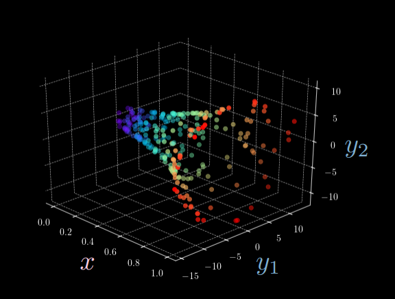
Figure 1: 3D Visualization of Ellipse Function

From Figure 1, it is clear that given a single input $x$, there are multiple possible output $\vect{y}$. In other words, we cannot identify a one-to-one mapping of vectors as we expected for Feed Forward Neural Networks (For example, there are almost always two possible $y_2$ fixing $y_1$ given input $x$). This is where we introduce the Latent Variable Energy-Based Models.

For simplicity, we fix input $x = 0$ and let $\alpha = 1.5, \beta = 2$, inducing \(\vect{y} = \begin{bmatrix} 2\cos(\theta) + \epsilon \\ 1.5\sin(\theta) + \epsilon \end{bmatrix}\) , from which we randomly sample 24 data points $Y = [\vect{y}^{(1)},\ldots,\vect{y}^{(24)}]$. Meanwhile, we take latent variable $z = [0:\frac{\pi}{24}:2\pi)$ and feed it into a decoder to produce $\tilde{\vect{y}}$ (Figure 2 and 3). Then, the energy function is computed as the squared Euclidean distance between $\vect{y}$ and $\tilde{\vect{y}}$:

where $\vect{g} = [g_1 \space\space g_2]^{\top} : \mathbb{R} \mapsto \mathbb{R}^2$ and $\vect{g}(z) = \ [w_1 \cos(z) \space\space w_2 \sin(z)]^{\top}$.

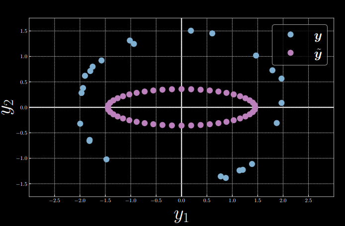
Figure 2: Sample Visualization

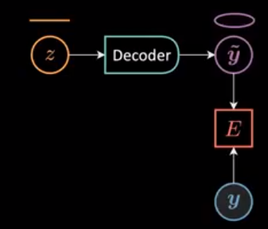
Figure 3: Energy Computation Graph

For each $\vect{y}^{(i)} \in Y, i \in [1,24]$, we can compute the corresponding energy given each $\tilde{\vect{y}}$ by changing $z$. Therefore, we may visualize 24 energy functions $E_{1},\ldots,E_{24}$, where energy quantity on y-axis is plotted against the choice of latent variable $z$ on the x-axis (Figure 4).

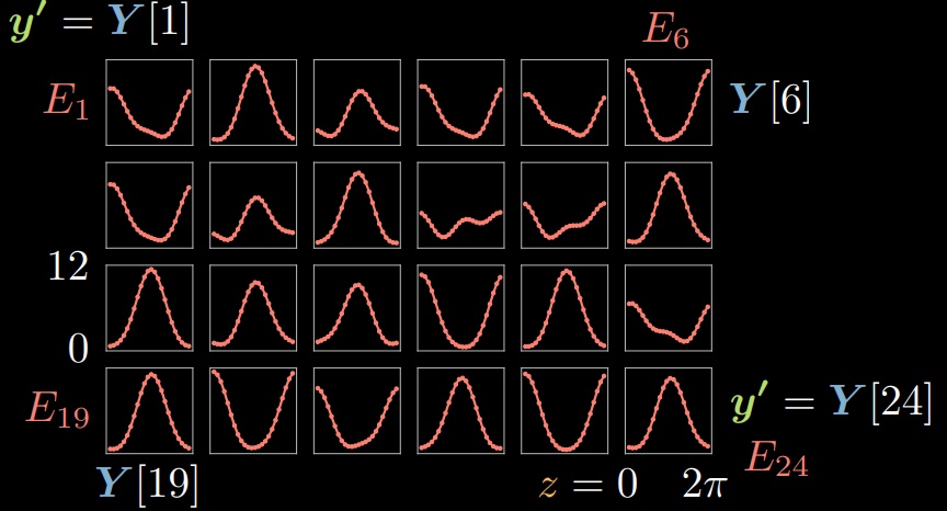
Figure 4: Energy Functions over Samples

Energy and free energy for two training samples

Let’s dive deeper into the functional form of the $E(\vect{y}, z)$ for a given $\vect{y}^{(i)}$. Figure 5 shows a plot of $E(\vect{y}^{(23)}, z) = E_{23}$.

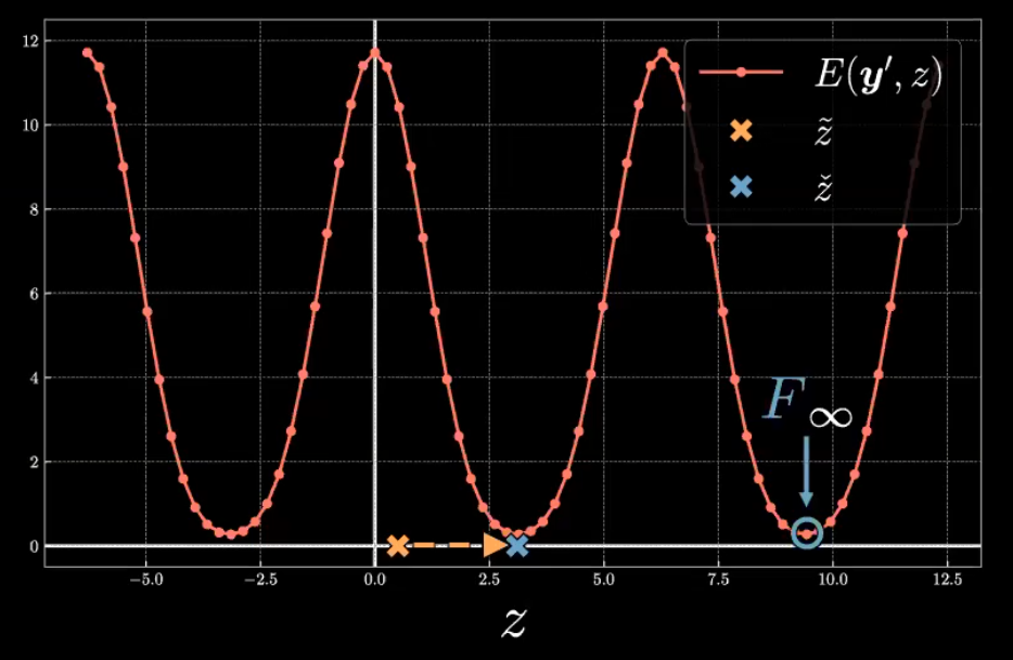
Figure 5: Energy Function associated with the 23rd Sample

Note that the energy, $E_{23}$, yields a periodic function with a maximum near $z=0$ and $2{\pi}$ and minimum near $z={\pi}$. This symmetric form arises due to the location $\vect{y}^{(23)}$ in the $\vect{y}$ space relative to the decoded $\tilde{\vect{y}}$.

As shown in Figure 6, $\vect{y}^{(23)}$ marked by the green point is closely aligned to the horizontal axis of $\tilde{\vect{y}}$ shown in purple which yields symmetry in $E_{23}$. The latent variable $z$ acts as a reverse polar coordinates angle such that the positive direction is clockwise. At $z=0$ (the leftmost purple point), the Euclidean distance between $\tilde{\vect{y}}$ and $\vect{y}^{(23)}$ is largely resulting in high energy. As $z$ approaches ${\pi}$ (the rightmost purple point), $\tilde{\vect{y}}$ gets closer to $\vect{y}^{(23)}$ which decreases the energy towards a minimum level. Conversely, as $z$ increases beyond ${\pi}$ towards $2{\pi}$, the distance between $\tilde{\vect{y}}$ and $\vect{y}^{(23)}$ increases, and hence the energy also increases towards a maximum.

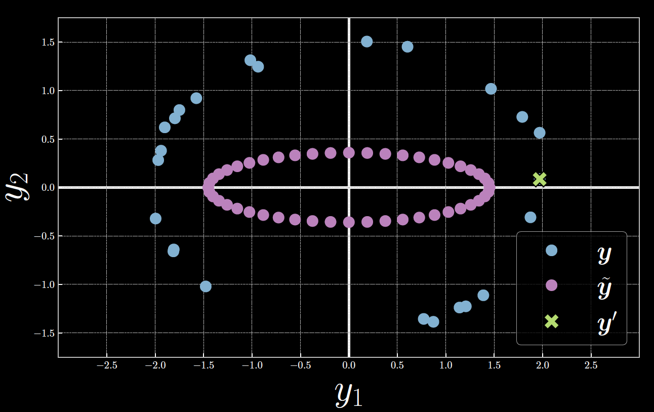
Figure 6: Relationship between Latent Variable, Decoder Output, and the 23rd Sample

Now that we have an understanding of the energy distribution, let’s evaluate the zero-temperature limit of the free energy defined by the following.

We will also express the latent variable which yields the free energy as $\check{z}$ defined by the following.

As depicted in Figure 5, to find the free energy associated with $\vect{y}^{(23)}$ we’ll start with an initial latent variable $\tilde{z}$. $\check{z}$ can be evaluated through optimization algorithms such as exhaustive search, conjugate gradient, line search, or limited-memory BFGS. The free energy is the minimum value of the energy with respect to the latent variable.

Figure 7 below shows the evaluation of the free energy in the $\vect{y}$ space. Note that throughout the optimization, the latent variable is increased such that $\tilde{\vect{y}}$ moves clockwise toward $\vect{y}^{(23)}$. At the free energy, the energy and consequently the distance between $\tilde{\vect{y}}$ and $\vect{y}^{(23)}$ is minimized.

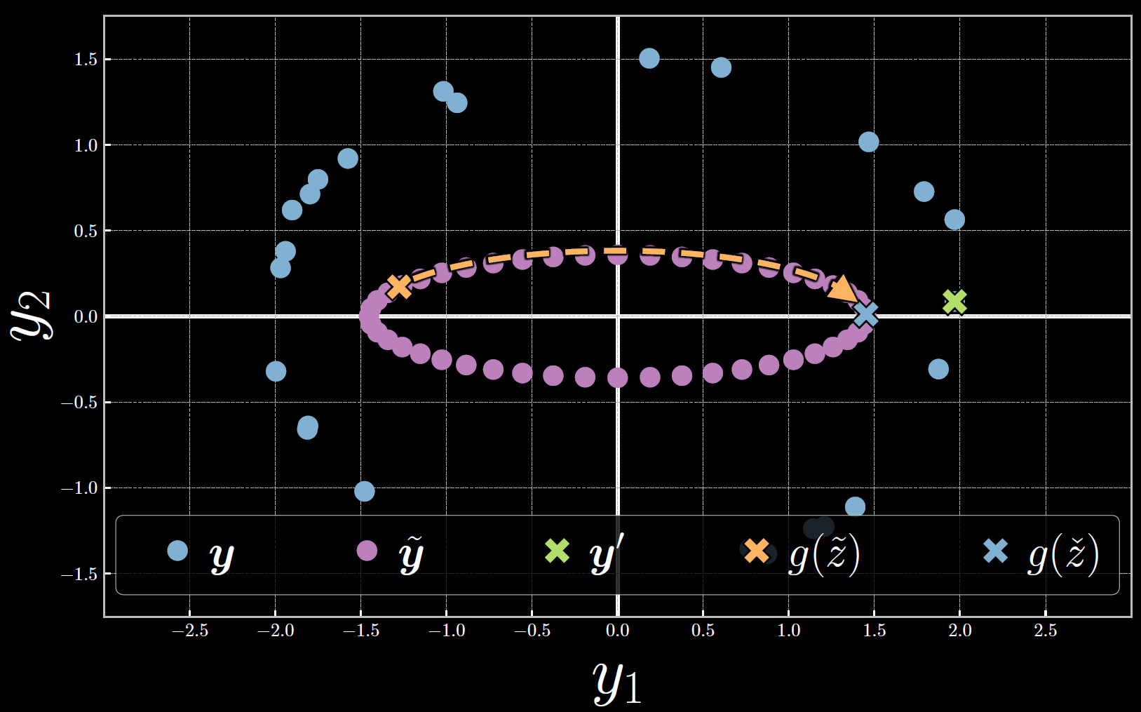
Figure 7: Free Energy Evaluation Associated with the 23rd Sample

In evaluating the free energy $F_\infty$ and its associated latent variable $\check{z}$, we are able to find the decoded $\tilde{\vect{y}}$ which is close to the sample data $\vect{y}^{(i)}$.

Free energy dense estimation

To understand the Free Energy Function better, we begin with the following example, shown in Figure 8.

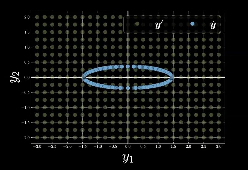
Figure 8: Free Energy Example in Mesh Grid

To compute the free energy, $F_\infty$, at each mesh grid point with respect to the manifold in blue color (which is also the all possible choices of the latent variables $z$), we first recall the definition of Free Energy Function as below:

Given the formula of the energy function, $E(\vect{y},z)$, and a location (sample) $\vect{y}$, our minimization process starts with inference, which is exactly the process to find the latent variable $\check{z}$ that most likely generates our location of sample. Graphically speaking with Figure 8, we start with an arbitrary point $z$ on the blue manifold and then move around the manifold to find the point, $\check{z}$, on the manifold that is closest to our sample location, $\vect{y}$. As a result, the free energy would be the Euclidean distance between our sample point $\vect{y}$ and the picked $\tilde{\vect{y}}(\check{z})$.

Now, we consider 5 specific sample points in the mesh grid, shown in Figure 9 with different colors.

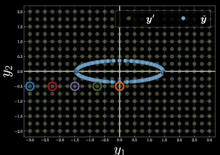
Figure 9: Five Sample Points on Mesh Grid

Utilizing what we learned above and give a guess to the energy function shapes of these five points, with respect to different choices of latent variable $z$ on the manifold. Exactly, the blue point will likely have energy function with the largest magnitude, and thus the largest free energy among the 5, and the orange point will likely have the smallest free energy.

The complete look of five energy functions given as following in Figure10, the cross signs represent the values of $\check{z}$ for each specific energy function.

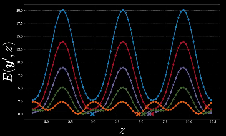
Figure 10: Energy Functions for the Five Points

Continuing the above example, we should note that our Free Energy Function, $F_\infty$, only takes non-negative scalar values for its range (because we are using Euclidean distance for $E(\vect{y},z)$), and the domain of our Free Energy Function, $F_\infty$, is $\mathbb{R}^2$ (only the $\vect{y}$ space), so generally we have $F_\infty :\mathbb{R}^2 \rightarrow \mathbb{R}^+$. We now use the free energy values as our inference to plot the above mesh grid as the following heat map, shown in Figure 11. To be noted, arrows represent gradient values.

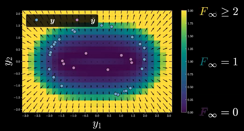
Figure 11: Free Energy Heat Map

To sum up, we only discuss a single example of Free Energy here. In real circumstances, we will have much wider choices of latent variables, $z$, rather than the only choice of ellipse manifold in our example. However, we need to keep in mind that the free energy value, $F_\infty$, is not dependent on the latent variable at all.

Comprehension Questions and Answers

Question 1: Why is the energy surface scalar-valued?

Energy surface, which takes the value of free energy, $F_\infty$, is exactly the minimum value of our energy function $E(\vect{y},z)$ across all possible latent variables, $z$. Therefore, $F_\infty$ is not dependent on $z$, but only on $\vect{y}$, which outputs a scalar value for each choice of $\vect{y}$.

Considering the mesh grid example above, the mesh grid has $17\times 25 = 425$ points, so we will have 425 free energy values, and each value is the quadratic Euclidean distance from each point to the manifold.

Question 2: How do you choose the function to represent the data manifold?

There are numerous researches about choices of the latent variable, and we may have a few layers of Neural Networks to represent the choices of latent variables.

One typical example is language translation. We can translate a sentence in different ways, and we may not use a softmax function for our model training as there will be infinitely many possible resulted sentences after translation. Therefore, we can use EBM here, and the energy function will tell how compatible is between our original sentence and translated sentence.

Question 3: Does minimizing energy regarding the trained manifold basically mean denoising?

If the model has learnt from the real manifold, then you can find the denoised version of your input by minimizing energy.