Activation and loss functions (part 1)

🎙️ Yann LeCun

Activation functions

In today’s lecture, we will review some important activation functions and their implementations in PyTorch. They came from various papers claiming these functions work better for specific problems.

ReLU - nn.ReLU()

\[\text{ReLU}(x) = (x)^{+} = \max(0,x)\]
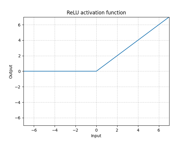
Fig. 1: ReLU

RReLU - nn.RReLU()

There are variations in ReLU. The Random ReLU (RReLU) is defined as follows.

\[\text{RReLU}(x) = \begin{cases} x, & \text{if} x \geq 0\\ ax, & \text{otherwise} \end{cases}\]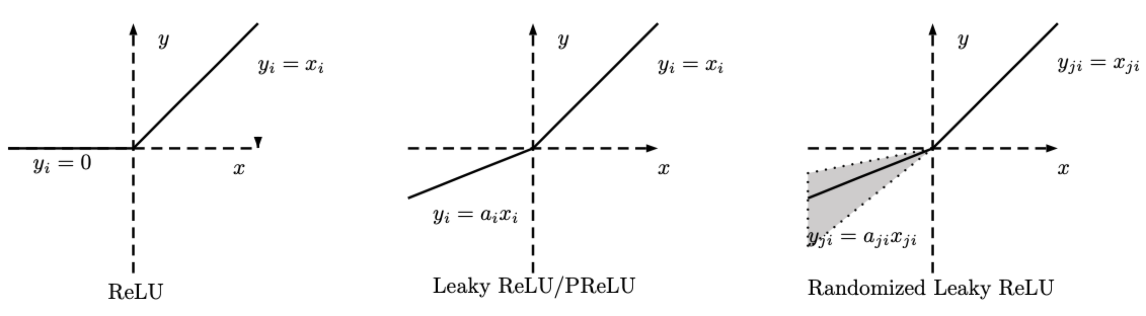
Fig. 2: ReLU, Leaky ReLU/PReLU, RReLU

Note that for RReLU, $a$ is a random variable that keeps samplings in a given range during training, and remains fixed during testing. For PReLU , $a$ is also learned. For Leaky ReLU, $a$ is fixed.

LeakyReLU - nn.LeakyReLU()

\[\text{LeakyReLU}(x) = \begin{cases} x, & \text{if} x \geq 0\\ a_\text{negative slope}x, & \text{otherwise} \end{cases}\]
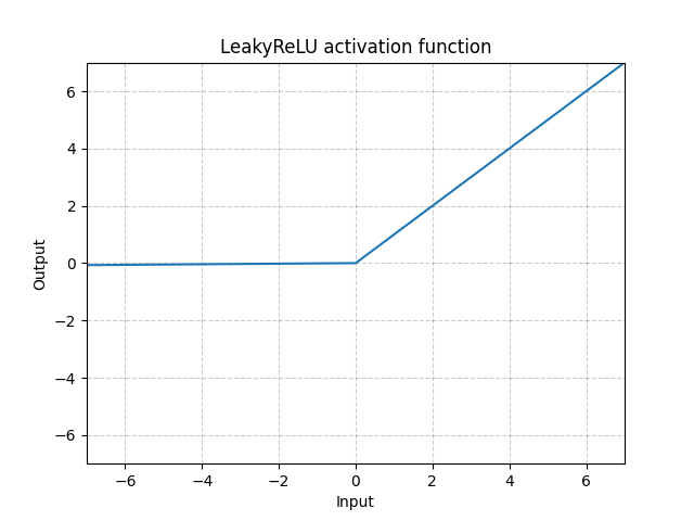
Fig. 3: LeakyReLU

Here $a$ is a fixed parameter. The bottom part of the equation prevents the problem of dying ReLU which refers to the problem when ReLU neurons become inactive and only output 0 for any input. Therefore, its gradient is 0. By using a negative slope, it allows the network to propagate back and learn something useful.

LeakyReLU is necessary for skinny network, which is almost impossible to get gradients flowing back with vanilla ReLU. With LeakyReLU, the network can still have gradients even we are in the region where everything is zero out.

PReLU - nn.PReLU()

\[\text{PReLU}(x) = \begin{cases} x, & \text{if} x \geq 0\\ ax, & \text{otherwise} \end{cases}\]

Here $a$ is a learnable parameter.

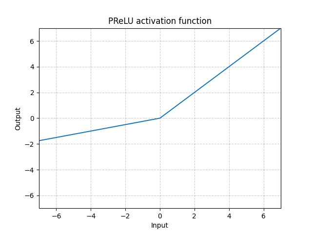
Fig. 4: ReLU

The above activation functions (i.e. ReLU, LeakyReLU, PReLU) are scale-invariant.

Softplus - Softplus()

\[\text{Softplus}(x) = \frac{1}{\beta} * \log(1 + \exp(\beta * x))\]
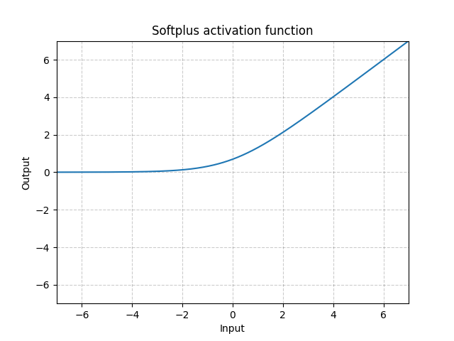
Fig. 5: Softplus

Softplus is a smooth approximation to the ReLU function and can be used to constrain the output of a machine to always be positive.

The function will become more like ReLU, if the $\beta$ gets larger and larger.

ELU - nn.ELU()

\[\text{ELU}(x) = \max(0, x) + \min(0, \alpha * (\exp(x) - 1)\]
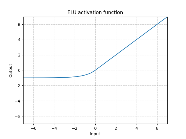
Fig. 6: ELU

Unlike ReLU, it can go below 0 which allows the system to have average output to be zero. Therefore, the model may converge faster. And its variations (CELU, SELU) are just different parametrizations.

CELU - nn.CELU()

\[\text{CELU}(x) = \max(0, x) + \min(0, \alpha * (\exp(x/\alpha) - 1)\]
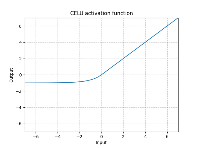
Fig. 7: CELU

SELU - nn.SELU()

\[\text{SELU}(x) = \text{scale} * (\max(0, x) + \min(0, \alpha * (\exp(x) - 1))\]
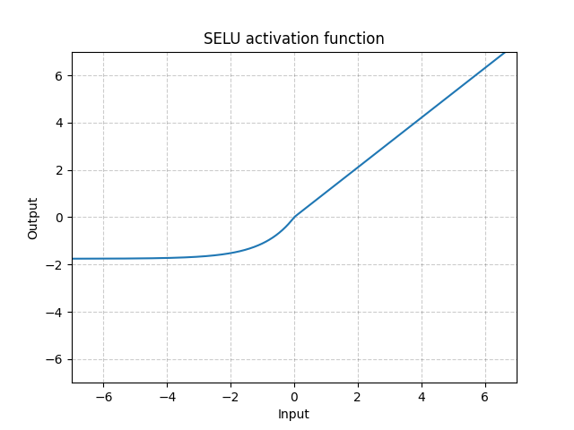
Fig. 8: SELU

GELU - nn.GELU()

\[\text{GELU(x)} = x * \Phi(x)\]

where $\Phi(x)$ is the Cumulative Distribution Function for Gaussian Distribution.

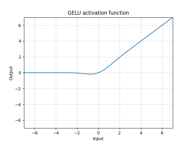
Fig. 9: GELU

ReLU6 - nn.ReLU6()

\[\text{ReLU6}(x) = \min(\max(0,x),6)\]
Fig. 10: ReLU6

This is ReLU saturating at 6. But there is no particular reason why picking 6 as saturation, so we can do better by using Sigmoid function below.

Sigmoid - nn.Sigmoid()

\[\text{Sigmoid}(x) = \sigma(x) = \frac{1}{1 + \exp(-x)}\]
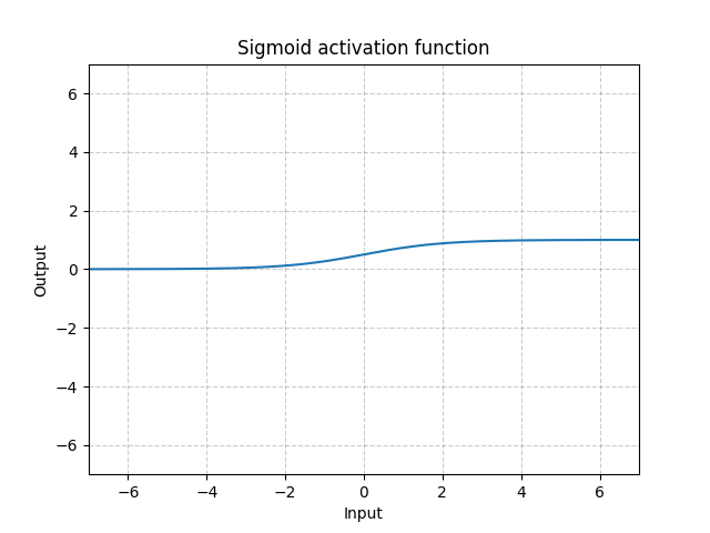
Fig. 11: Sigmoid

If we stack sigmoids in many layers, it may be inefficient for the system to learn and requires careful initialization. This is because if the input is very large or small, the gradient of the sigmoid function is close to 0. In this case, there is no gradient flowing back to update the parameters, known as saturating gradient problem. Therefore, for deep neural networks, a single kink function (such as ReLU) is preferred.

Tanh - nn.Tanh()

\[\text{Tanh}(x) = \tanh(x) = \frac{\exp(x) - \exp(-x)}{\exp(x) + \exp(-x)}\]
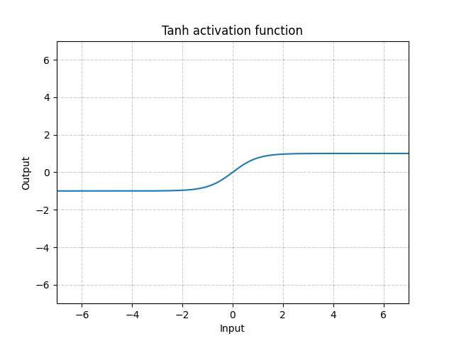
Fig. 12: Tanh

Tanh is basically identical to Sigmoid except it is centred, ranging from -1 to 1. The output of the function will have roughly zero mean. Therefore, the model will converge faster. Note that convergence is usually faster if the average of each input variable is close to zero. One example is Batch Normalization.

Softsign - nn.Softsign()

\[\text{SoftSign}(x) = \frac{x}{1 + |x|}\]
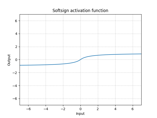
Fig. 13: Softsign

It is similar to the Sigmoid function but gets to the asymptote slowly and alleviate the gradient vanishing problem (to some extent).

Hardtanh - nn.Hardtanh()

\[\text{HardTanh}(x) = \begin{cases} 1, & \text{if} x > 1\\ -1, & \text{if} x < -1\\ x, & \text{otherwise} \end{cases}\]

The range of the linear region [-1, 1] can be adjusted using min_val and max_val.

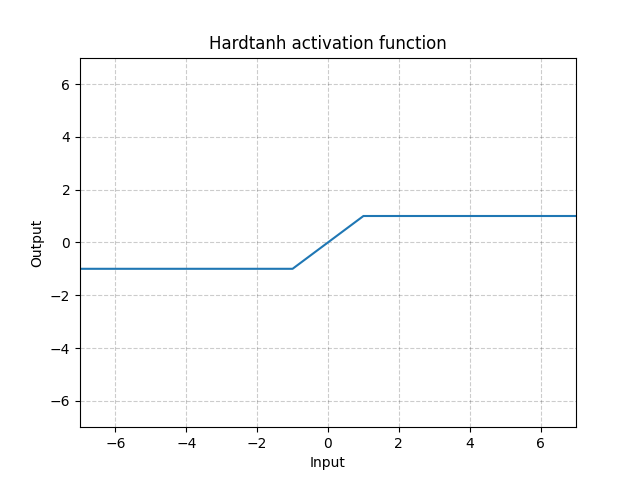
Fig. 14: Hardtanh

It works surprisingly well especially when weights are kept within the small value range.

Threshold - nn.Threshold()

\[y = \begin{cases} x, & \text{if} x > \text{threshold}\\ v, & \text{otherwise} \end{cases}\]

It is rarely used because we cannot propagate the gradient back. And it is also the reason preventing people from using back-propagation in 60s and 70s when they were using binary neurons.

Tanhshrink - nn.Tanhshrink()

\[\text{Tanhshrink}(x) = x - \tanh(x)\]
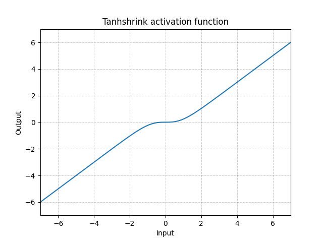
Fig. 15: Tanhshrink

It is rarely used except for sparse coding to compute the value of the latent variable.

Softshrink - nn.Softshrink()

\[\text{SoftShrinkage}(x) = \begin{cases} x - \lambda, & \text{if} x > \lambda\\ x + \lambda, & \text{if} x < -\lambda\\ 0, & \text{otherwise} \end{cases}\]
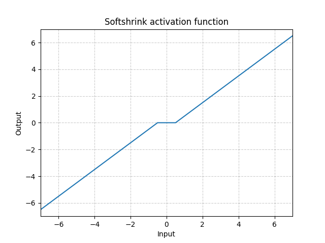
Fig. 16: Softshrink

This basically shrinks the variable by a constant towards 0, and forces to 0 if the variable is close to 0. You can think of it as a step of gradient for the $\ell_1$ criteria. It is also one of the step of the Iterative Shrinkage-Thresholding Algorithm (ISTA). But it is not commonly used in standard neural network as activations.

Hardshrink - nn.Hardshrink()

\[\text{HardShrinkage}(x) = \begin{cases} x, & \text{if} x > \lambda\\ x, & \text{if} x < -\lambda\\ 0, & \text{otherwise} \end{cases}\]
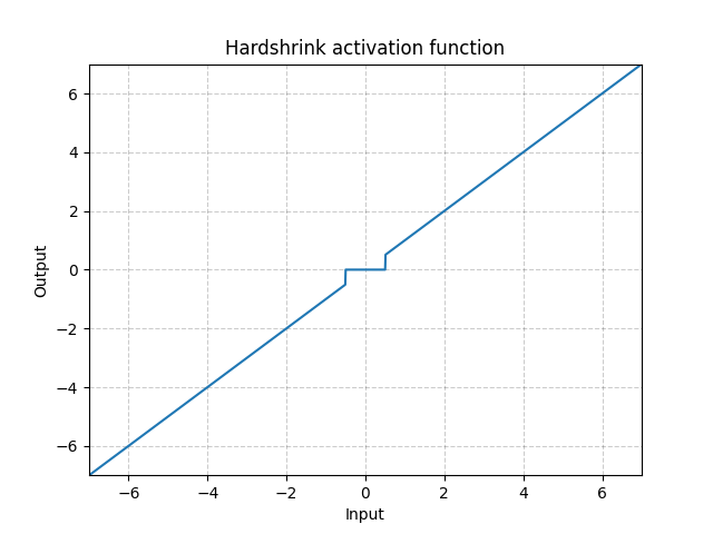
Fig. 17: Hardshrink

It is rarely used except for sparse coding.

LogSigmoid - nn.LogSigmoid()

\[\text{LogSigmoid}(x) = \log\left(\frac{1}{1 + \exp(-x)}\right)\]
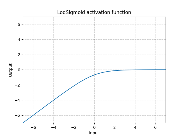
Fig. 18: LogSigmoid

It is mostly used in the loss function but not common for activations.

Softmin - nn.Softmin()

\[\text{Softmin}(x_i) = \frac{\exp(-x_i)}{\sum_j \exp(-x_j)}\]

It turns numbers into a probability distribution.

Soft(arg)max - nn.Softmax()

\[\text{Softmax}(x_i) = \frac{\exp(x_i)}{\sum_j \exp(x_j)}\]

LogSoft(arg)max - nn.LogSoftmax()

\[\text{LogSoftmax}(x_i) = \log\left(\frac{\exp(x_i)}{\sum_j \exp(x_j)}\right)\]

It is mostly used in the loss function but not common for activations.

Q&A activation functions

nn.PReLU() related questions

• Why would we want the same value of $a$ for all channels?

  Different channels could have different $a$. You could use $a$ as a parameter of every unit. It could be shared as a feature map as well.

• Do we learn $a$? Is learning $a$ advantageous?

  You can learn $a$ or fix it. The reason for fixing is to ensure that nonlinearity gives you a non-zero gradient even if it’s in a negative region. Making $a$ learnable allows the system to turn nonlinearity into either linear mapping or full rectification. It could be useful for some applications like implementing an edge detector regardless of the edge polarity.

• How complex do you want your non-linearity to be?

  Theoretically, we can parametrise an entire nonlinear function in very complicated way, such as with spring parameters, Chebyshev polynomial, etc. Parametrising could be a part of learning process.

• What is an advantage of parametrising over having more units in your system?

  It really depends on what you want to do. For example, when doing regression in a low dimensional space, parametrisation might help. However, if your task is in under a high dimensional space such as image recognition, just “a” nonlinearity is necessary and monotonic nonlinearity will work better. In short, you can parametrize any functions you want but it doesn’t bring a huge advantage.

Kink related questions

• One kink versus double kink

  Double kink is a built-in scale in it. This means that if the input layer is multiplied by two (or the signal amplitude is multiplied by two), then outputs will be completely different. The signal will be more in nonlinearity, thus you will get a completely different behaviour of the output. Whereas, if you have a function with only one kink, if you multiply the input by two, then your output will be also multiplied by two.

• Differences between a nonlinear activation having kinks and a smooth nonlinear activation. Why/when one of them is preferred?

  It is a matter of scale equivariance. If kink is hard, you multiply the input by two and the output is multiplied by two. If you have a smooth transition, for example, if you multiply the input by 100, the output looks like you have a hard kink because the smooth part is shrunk by a factor of 100. If you divide the input by 100, the kink becomes a very smooth convex function. Thus, by changing the scale of the input, you change the behaviour of the activation unit.

  Sometimes this could be a problem. For example, when you train a multi-layer neural net and you have two layers that are one after the other. You do not have a good control for how big the weights of one layer is relative to the other layer’s weights. If you have nonlinearity that cares about scales, your network doesn’t have a choice of what size of weight matrix can be used in the first layer because this will completely change the behaviour.

  One way to fix this problem is setting a hard scale on the weights of every layer so you can normalise the weights of layers, such as batch normalisation. Thus, the variance that goes into a unit becomes always constant. If you fix the scale, then the system doesn’t have any way of choosing which part of the nonlinearity will be using in two kink function systems. This could be a problem if this ‘fixed’ part becomes too ‘linear’. For example, Sigmoid becomes almost linear near zero, and thus batch normalisation outputs (close to 0) could not be activated ‘non-linearly’.

  It is not entirely clear why deep networks work better with single kink functions. It’s probably due to the scale equivariance property.

Temperature coefficient in a soft(arg)max function

• When do we use the temperature coefficient and why do we use it?

  To some extent, the temperature is redundant with incoming weights. If you have weighted sums coming into your softmax, the $\beta$ parameter is redundant with the size of weights.

  Temperature controls how hard the distribution of output will be. When $\beta$ is very large, it becomes very close to either one or zero. When $\beta$ is small, it is softer. When the limit of $\beta$ equals to zero, it is like an average. When $\beta$ goes infinity, it behaves like argmax. It’s no longer its soft version. Thus, if you have some sort of normalisation before the softmax then, tuning this parameter allows you to control the hardness. Sometimes, you can start with a small $\beta$ so that you can have well-behaved gradient descents and then, as running proceeds, if you want a harder decision in your attention mechanism, you increase $\beta$. Thus, you can sharpen the decisions. This trick is called as annealing. It can be useful for a mixture of experts like a self attention mechanism.

Loss functions

PyTorch also has a lot of loss functions implemented. Here we will go through some of them.

nn.MSELoss()

This function gives the mean squared error (squared L2 norm) between each element in the input $x$ and target $y$. It is also called L2 loss.

If we are using a minibatch of $n$ samples, then there are $n$ losses, one for each sample in the batch. We can tell the loss function to keep that loss as a vector or to reduce it.

If unreduced (i.e. set reduction='none'), the loss is

\[l(x,y) = L = \{l_1, \dots, l_N\}^\top, l_n = (x_n - y_n)^2\]

where $N$ is the batch size, $x$ and $y$ are tensors of arbitrary shapes with a total of n elements each.

The reduction options are below (note that the default value is reduction='mean').

\[l(x,y) = \begin{cases}\text{mean}(L), \quad &\text{if reduction='mean'}\\ \text{sum}(L), \quad &\text{if reduction='sum'} \end{cases}\]

The sum operation still operates over all the elements, and divides by $n$.

The division by $n$ can be avoided if one sets reduction = 'sum'.

nn.L1Loss()

This measures the mean absolute error (MAE) between each element in the input $x$ and target $y$ (or the actual output and desired output).

If unreduced (i.e. set reduction='none'), the loss is

\[l(x,y) = L = \{l_1, \dots, l_N\}^\top, l_n = \vert x_n - y_n\vert\]

, where $N$ is the batch size, $x$ and $y$ are tensors of arbitrary shapes with a total of n elements each.

It also has reduction option of 'mean' and 'sum' similar to what nn.MSELoss() have.

Use Case: L1 loss is more robust against outliers and noise compared to L2 loss. In L2, the errors of those outlier/noisy points are squared, so the cost function gets very sensitive to outliers.

Problem: The L1 loss is not differentiable at the bottom (0). We need to be careful when handling its gradients (namely Softshrink). This motivates the following SmoothL1Loss.

nn.SmoothL1Loss()

This function uses L2 loss if the absolute element-wise error falls below 1 and L1 loss otherwise.

\(\text{loss}(x, y) = \frac{1}{n} \sum_i z_i\) , where $z_i$ is given by

\[z_i = \begin{cases}0.5(x_i-y_i)^2, \quad &\text{if } |x_i - y_i| < 1\\ |x_i - y_i| - 0.5, \quad &\text{otherwise} \end{cases}\]

It also has reduction options.

This is advertised by Ross Girshick (Fast R-CNN). The Smooth L1 Loss is also known as the Huber Loss or the Elastic Network when used as an objective function,.

Use Case: It is less sensitive to outliers than the MSELoss and is smooth at the bottom. This function is often used in computer vision for protecting against outliers.

Problem: This function has a scale ($0.5$ in the function above).

L1 vs. L2 for Computer Vision

In making predictions when we have a lot of different $y$’s:

• If we use MSE (L2 Loss), it results in an average of all $y$, which in CV it means we will have a blurry image.
• If we use L1 loss, the value $y$ that minimize the L1 distance is the medium, which is not blurry, but note that medium is difficult to define in multiple dimensions.

Using L1 results in sharper image for prediction.

nn.NLLLoss()

It is the negative log likelihood loss used when training a classification problem with C classes.

Note that, mathematically, the input of NLLLoss should be (log) likelihoods, but PyTorch doesn’t enforce that. So the effect is to make the desired component as large as possible.

The unreduced (i.e. with :attr:reduction set to 'none') loss can be described as:

\[\ell(x, y) = L = \{l_1,\dots,l_N\}^\top, \quad l_n = - w_{y_n} x_{n,y_n}, \quad w_{c} = \text{weight}[c] \cdot \mathbb{1}\{c \not= \text{ignore\_index}\}\]

,where $N$ is the batch size.

If reduction is not 'none' (default 'mean'), then

\[\ell(x, y) = \begin{cases} \sum_{n=1}^N \frac{1}{\sum_{n=1}^N w_{y_n}} l_n, & \text{if reduction} = \text{'mean';}\\ \sum_{n=1}^N l_n, & \text{if reduction} = \text{'sum'.} \end{cases}\]

This loss function has an optional argument weight that can be passed in using a 1D Tensor assigning weight to each of the classes. This is useful when dealing with imbalanced training set.

Weights & Imbalanced Classes:

Weight vector is useful if the frequency is different for each category/class. For example, the frequency of the common flu is much higher than the lung cancer. We can simply increase the weight for categories that has small number of samples.

However, instead of setting the weight, it’s better to equalize the frequency in training so that we can exploits stochastic gradients better.

To equalize the classes in training, we put samples of each class in a different buffer. Then generate each minibatch by picking the same number samples from each buffer. When the smaller buffer runs out of samples to use, we iterate through the smaller buffer from the beginning again until every sample of the larger class is used. This way gives us equal frequency for all categories by going through those circular buffers. We should never go the easy way to equalize frequency by not using all samples in the majority class. Don’t leave data on the floor!

An obvious problem of the above method is that our NN model wouldn’t know the relative frequency of the actual samples. To solve that, we fine-tune the system by running a few epochs at the end with the actual class frequency, so that the system adapts to the biases at the output layer to favour things that are more frequent.

To get an intuition of this scheme, let’s go back to the medical school example: students spend just as much time on rare disease as they do on frequent diseases (or maybe even more time, since the rare diseases are often the more complex ones). They learn to adapt to the features of all of them, then correct it to know which are rare.

nn.CrossEntropyLoss()

This function combines nn.LogSoftmax and nn.NLLLoss in one single class. The combination of the two makes the score of the correct class as large as possible.

The reason why the two functions are merged here is for numerical stability of gradient computation. When the value after softmax is close to 1 or 0, the log of that can get close to 0 or $-\infty$. Slope of log close to 0 is close to $\infty$, causing the intermediate step in backpropagation to have numerical issues. When the two functions are combined, the gradients is saturated so we get a reasonable number at the end.

The input is expected to be unnormalised score for each class.

The loss can be described as:

\[\text{loss}(x, c) = -\log\left(\frac{\exp(x[c])}{\sum_j \exp(x[j])}\right) = -x[c] + \log\left(\sum_j \exp(x[j])\right)\]

or in the case of the weight argument being specified:

\[\text{loss}(x, c) = w[c] \left(-x[c] + \log\left(\sum_j\exp(x[j])\right)\right)\]

The losses are averaged across observations for each minibatch.

A physical interpretation of the Cross Entropy Loss is related to the Kullback–Leibler divergence (KL divergence), where we are measuring the divergence between two distributions. Here, the (quasi) distributions are represented by the x vector (predictions) and the target distribution (a one-hot vector with 0 on the wrong classes and 1 on the right class).

Mathematically,

\[H(p,q) = H(p) + \mathcal{D}_{KL} (p \mid\mid q)\]

where \(H(p,q) = - \sum_i p(x_i) \log (q(x_i))\) is the cross-entropy (between two distributions), \(H(p) = - \sum_i p(x_i) \log (p(x_i))\) is the entropy, and \(\mathcal{D}_{KL} (p \mid\mid q) = \sum_i p(x_i) \log \frac{p(x_i)}{q(x_i)}\) is the KL divergence.

nn.AdaptiveLogSoftmaxWithLoss()

This is an efficient softmax approximation of softmax for large number of classes (for example, millions of classes). It implements tricks to improve the speed of the computation.

Details of the method is described in Efficient softmax approximation for GPUs by Edouard Grave, Armand Joulin, Moustapha Cissé, David Grangier, Hervé Jégou.

---

📝 Haochen Wang, Eunkyung An, Ying Jin, Ningyuan Huang
13 April 2020