Artificial neural networks (ANNs)

🎙️ Alfredo Canziani

Supervised learning for classification

• Consider Fig. 1(a) below. The points in this graph lie on the branches of the spiral, and live in $\R^2$. Each colour represents a class label. The number of unique classes is $K = 3$. This is represented mathematically by Eqn. 1(a).

• Fig. 1(b) shows a similar spiral, with an added Gaussian noise term. This is represented mathematically by Eqn. 1(b).

  In both cases, these points are not linearly separable.

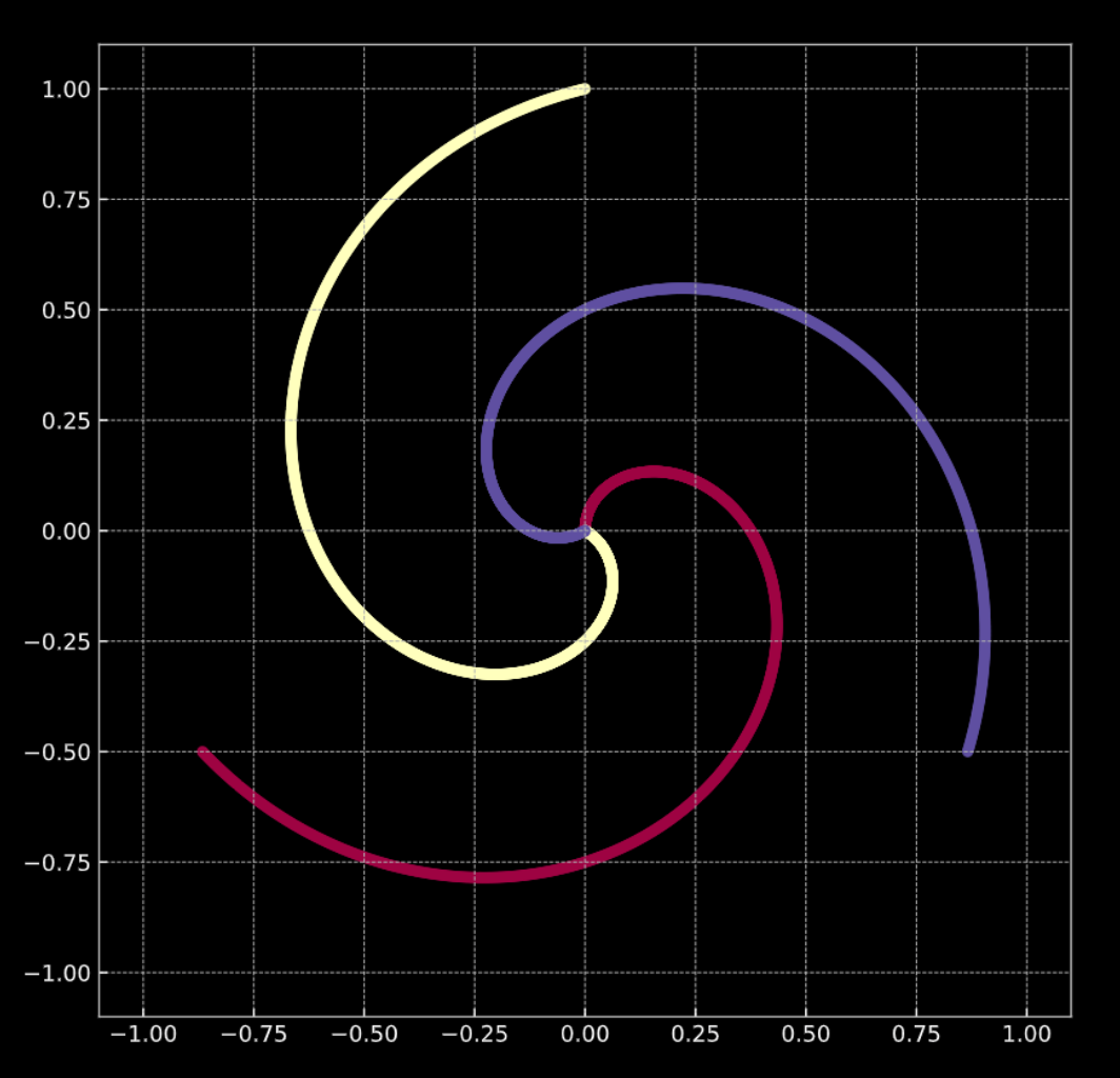
  Fig. 1(a) "Clean" 2D spiral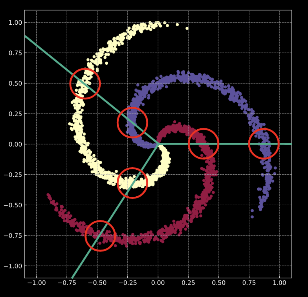

  Fig. 1(b) "Noisy" 2D spiral

\[X_{k}(t)=t\left(\begin{array}{c}{\sin \left[\frac{2 \pi}{K}(2 t+k-1)\right]} \\ {\cos \left[\frac{2 \pi}{K}(2 t+k-1)\right]}\end{array}\right) \\ 0 \leq t \leq 1, \quad k=1, ..., K\] Eqn. 1(a) \[X_{k}(t)=t\left(\begin{array}{c}{\sin \left[\frac{2 \pi}{K}(2 t+k-1 +\mathcal{N}\left(0, \sigma^{2}\right))\right]} \\ {\cos \left[\frac{2 \pi}{K}(2 t+k-1 +\mathcal{N}\left(0, \sigma^{2}\right))\right]}\end{array}\right)\\0 \leq t \leq 1, \quad k=1, ..., K\] Eqn. 1(b)

What does it mean to perform classification? Consider the case of logistic regression. If logistic regression for classification is applied to this data, it will create a set of linear planes (decision boundaries) in an attempt to separate the data into its classes. The issue with this solution is that in each region, there are points belonging to multiple classes. The branches of the spiral cross the linear decision boundaries. This is not a great solution!

How do we fix this? We transform the input space such that the data are forced to be linearly separable. Over the course of training a neural network to do this, the decision boundaries that it learns will try to adapt to the distribution of the training data.

Note: A neural network is always represented from the bottom up. The first layer is at the bottom, and the last at the top. This is because conceptually, the input data are low-level features for whatever task the neural network is attempting. As the data traverse upward through the network, each subsequent layer extracts features at a higher level.

Training data

Last week, we saw that a newly initialised neural network transforms its input in an arbitrary way. This transformation, however, isn’t (initially) instrumental in performing the task at hand. We explore how, using data, we can force this transformation to have some meaning that is relevant to the task at hand. The following are data used as training input for a network.

• $\vect{X}$ represents the input data, a matrix of dimensions $m$ (number of training data points) x $n$ (dimensionality of each input point). In case of the data shown in Figures 1(a) and 1(b), $n = 2$.

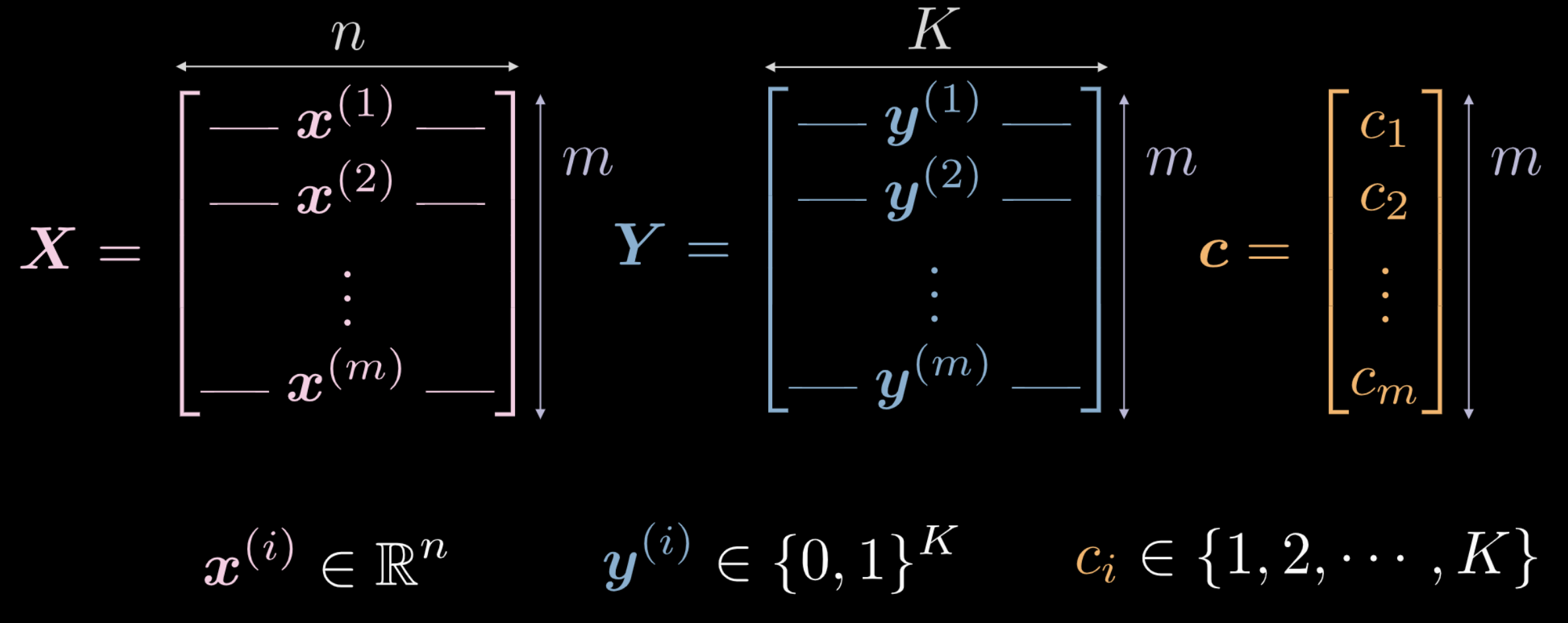
Fig. 2 Training data

• Vector $\vect{c}$ and matrix $\boldsymbol{Y}$ both represent class labels for each of the $m$ data points. In the example above, there are $3$ distinct classes.

  • $c_i \in \lbrace 1, 2, \cdots, K \rbrace$, and $\vect{c} \in \R^m$. However, we may not use $\vect{c}$ as training data. If we use distinct numeric class labels $c_i \in \lbrace 1, 2, \cdots, K \rbrace$, the network may infer an order within the classes that isn’t representative of the data distribution.
  • To bypass this issue, we use a one-hot encoding. For each label $c_i$, a $K$ dimensional zero-vector $\vect{y}^{(i)}$ is created, which has the $c_i$-th element set to $1$ (see Fig. 3 below).

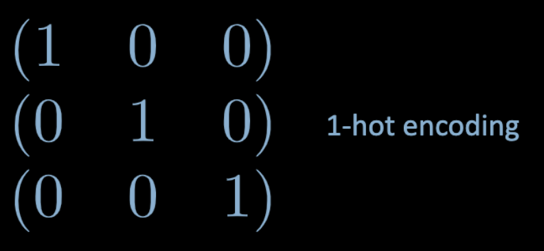
Fig. 3 One hot encoding

• Therefore, $\boldsymbol Y \in \R^{m \times K}$. This matrix can also be thought of as having some probabilistic mass, which is fully concentrated on one of the $K$ spots.

Fully (FC) connected layers

We will now take a look at what a fully connected (FC) network is, and how it works.

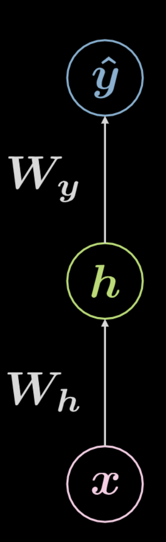
Fig. 4 Fully connected neural network

Consider the network shown above in Fig. 4. The input data, $\boldsymbol x$, is subject to an affine transformation defined by $\boldsymbol W_h$, followed by a non-linear transformation. The result of this non-linear transformation is denoted as $\boldsymbol h$, representing a hidden output, i.e one that is not seen from outside the network. This is followed by another affine transformation ($\boldsymbol W_y$), followed by another non-linear transformation. This produces the final output, $\boldsymbol{\hat{y}}$. This network can be represented mathematically by the equations in Eqn. 2 below. $f$ and $g$ are both non-linearities.

\[\begin{aligned} &\boldsymbol h=f\left(\boldsymbol{W}_{h} \boldsymbol x+ \boldsymbol b_{h}\right)\\ &\boldsymbol{\hat{y}}=g\left(\boldsymbol{W}_{y} \boldsymbol h+ \boldsymbol b_{y}\right) \end{aligned}\] Eqn. 2 Mathematics behind a FC network

A basic neural network such as the one shown above is merely a set of successive pairs, with each pair being an affine transformation followed by a non-linear operation (squashing). Frequently used non-linear functions include ReLU, sigmoid, hyperbolic tangent, and softmax.

The network shown above is a 3-layer network:

1. input neuron
2. hidden neuron
3. output neuron

Therefore, a $3$-layer neural network has $2$ affine transformations. This can be extended to a $n$-layer network.

Now let’s move to a more complicated case.

Let’s do a case of 3 hidden layers, fully connected in each layer. An illustration can be found in Fig. 5

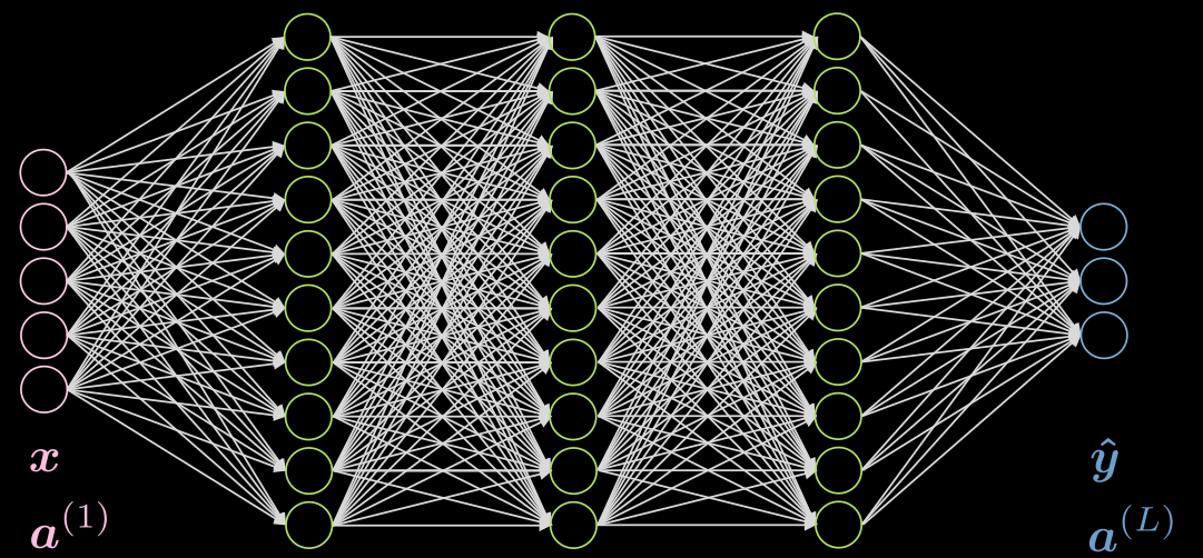
Fig. 5 Neural net with 3 hidden layers

Let’s consider a neuron $j$ in the second layer. It’s activation is:

\[a^{(2)}_j = f(\boldsymbol w^{(j)} \boldsymbol x + b_j) = f\Big( \big(\sum_{i=1}^n w_i^{(j)} x_i\big) +b_j ) \Big)\]

where $\vect{w}^{(j)}$ is the $j$-th row of $\vect{W}^{(1)}$.

Notice that the activation of the input layer in this case is just the identity. The hidden layers can have activations like ReLU, hyperbolic tangent, sigmoid, soft (arg)max, etc.

The activation of the last layer in general would depend on your use case, as explained in this Piazza post.

Neural network (inference)

Let’s think about the three-layer (input, hidden, output) neural network again, as seen in Fig. 6

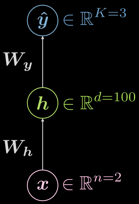
Fig. 6 Three-layer neural network

What kind of functions are we looking at?

\[\boldsymbol {\hat{y}} = \boldsymbol{\hat{y}(x)}, \boldsymbol{\hat{y}}: \mathbb{R}^n \rightarrow \mathbb{R}^K, \boldsymbol{x} \mapsto \boldsymbol{\hat{y}}\]

However, it is helpful to visualize the fact that there is a hidden layer, and the mapping can be expanded as:

\[\boldsymbol{\hat{y}}: \mathbb{R}^{n} \rightarrow \mathbb{R}^d \rightarrow \mathbb{R}^K, d \gg n, K\]

What might an example configuration for the case above look like? In this case, one has input of dimension two ($n=2$), the single hidden layer could have dimensionality of 1000 ($d = 1000$), and we have 3 classes ($C=3$). There are good practical reasons to not have so many neurons in one hidden layer, so it could make sense to split that single hidden layer into 3 with 10 neurons each ($1000 \rightarrow 10 \times 10 \times 10$).

Neural network (training I)

So what does typical training look like? It is helpful to formulate this into the standard terminology of losses.

First, let us re-introduce the soft (arg)max and explicitly state that it is a common activation function for the last layer, when using negative log-likelihood loss, in cases for multi-class prediction. As stated by Professor LeCun in lecture, this is because you get nicer gradients than if you were to use sigmoids and square loss. In addition, your last layer will already be normalized (the sum of all the neurons in the last layer come out to 1), in a way that is nicer for gradient methods than explicit normalization (dividing by the norm).

The soft (arg)max will give you logits in the last layer that look like this:

\[\text{soft{(arg)}max}(\boldsymbol{l})[c] = \frac{ \exp(\boldsymbol{l}[c])} {\sum^K_{k=1} \exp(\boldsymbol{l}[k])} \in (0, 1)\]

It is important to note that the set is not closed because of the strictly positive nature of the exponential function.

Given the set of the predictions $\matr{\hat{Y}}$, the loss will be:

\[\mathcal{L}(\boldsymbol{\hat{Y}}, \boldsymbol{c}) = \frac{1}{m} \sum_{i=1}^m \ell(\boldsymbol{\hat{y}_i}, c_i), \quad \ell(\boldsymbol{\hat{y}}, c) = -\log(\boldsymbol{\hat{y}}[c])\]

Here $c$ denotes the integer label, not the one hot encoding representation.

So let’s do two examples, one where an example is correctly classified, and one where it is not.

Let’s say

\[\boldsymbol{x}, c = 1 \Rightarrow \boldsymbol{y} = {\footnotesize\begin{pmatrix} 1 \\ 0 \\ 0 \end{pmatrix}}\]

What is the instance wise loss?

For the case of nearly perfect prediction ($\sim$ means circa):

\[\hat{\boldsymbol{y}}(\boldsymbol{x}) = {\footnotesize\begin{pmatrix} \sim 1 \\ \sim 0 \\ \sim 0 \end{pmatrix}} \Rightarrow \ell \left( {\footnotesize\begin{pmatrix} \sim 1 \\ \sim 0 \\ \sim 0 \end{pmatrix}} , 1\right) \rightarrow 0^{+}\]

For the case of nearly absolutely wrong:

\[\hat{\boldsymbol{y}}(\boldsymbol{x}) = {\footnotesize\begin{pmatrix} \sim 0 \\ \sim 1 \\ \sim 0 \end{pmatrix}} \Rightarrow \ell \left( {\footnotesize\begin{pmatrix} \sim 0 \\ \sim 1 \\ \sim 0 \end{pmatrix}} , 1\right) \rightarrow +\infty\]

Note in the above examples, $\sim 0 \rightarrow 0^{+}$ and $\sim 1 \rightarrow 1^{-}$. Why is this so? Take a minute to think.

Note: It is important to know that if you use CrossEntropyLoss, you will get LogSoftMax and negative loglikelihood NLLLoss bundled together, so don’t do it twice!

Neural network (training II)

For training, we aggregate all trainable parameters – weight matrices and biases – into a collection we call $\mathbf{\Theta} = \lbrace\boldsymbol{W_h, b_h, W_y, b_y} \rbrace$. This allows us to write the objective function or loss as:

\[J \left( \mathbf{\Theta} \right) = \mathcal{L} \left( \boldsymbol{\hat{Y}} \left( \mathbf{\Theta} \right), \boldsymbol c \right) \in \mathbb{R}^{+}\]

This makes the loss depend on the output of the network $\boldsymbol {\hat{Y}} \left( \mathbf{\Theta} \right)$, so we can turn this into an optimization problem.

A simple illustration of how this works can be seen in Fig. 7, where $J(\vartheta)$, the function we need to minimise, has only a scalar parameter $\vartheta$.

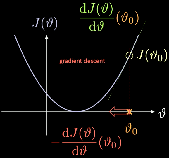
Fig. 7 Optimizing a loss function through gradient descent.

We pick a random initialization point $\vartheta_0$ – with associated loss $J(\vartheta_0)$. We can compute the derivative evaluated at that point $J’(\vartheta_0) = \frac{\text{d} J(\vartheta)}{\text{d} \vartheta} (\vartheta_0)$. In this case, the slope of the derivative is positive. So we need to take a step in the direction of steepest descent. In this case, that is $-\frac{\text{d} J(\vartheta)}{\text{d} \vartheta}(\vartheta_0)$.

The iterative repetition of this process is known as gradient descent. Gradient methods are the primary tools to train a neural network.

In order to compute the necessary gradients, we have to use back-propagation

\[\frac{\partial \, J(\mathbf{\Theta})}{\partial \, \boldsymbol{W_y}} = \frac{\partial \, J(\mathbf{\Theta})}{\partial \, \boldsymbol{\hat{y}}} \; \frac{\partial \, \boldsymbol{\hat{y}}}{\partial \, \boldsymbol{W_y}} \quad \quad \quad \frac{\partial \, J(\mathbf{\Theta})}{\partial \, \boldsymbol{W_h}} = \frac{\partial \, J(\mathbf{\Theta})}{\partial \, \boldsymbol{\hat{y}}} \; \frac{\partial \, \boldsymbol{\hat{y}}}{\partial \, \boldsymbol h} \;\frac{\partial \, \boldsymbol h}{\partial \, \boldsymbol{W_h}}\]

Spiral classification - Jupyter notebook

The Jupyter notebook can be found here. In order to run the notebook, make sure you have the dl-minicourse environment installed as specified in README.md.

An explanation of how to use torch.device() can be found in last week’s notes.

Like before, we are going to be working with points in $\mathbb{R}^2$ with three different categorical labels – in red, yellow and blue – as can be seen in Fig. 8.

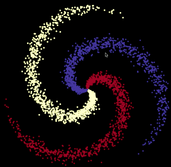
Fig. 8 Spiral classification data.

nn.Sequential() is a container, which passes modules to the constructor in the order that they are added; nn.linear() is miss-named as it applies an affine transformation to the incoming data: $\boldsymbol y = \boldsymbol W \boldsymbol x + \boldsymbol b$. For more information, refer to the PyTorch documentation.

Remember, an affine transformation is five things: rotation, reflection, translation, scaling and shearing.

As it can be seen in Fig. 9, when trying to separate the spiral data with linear decision boundaries - only using nn.linear() modules, without a non-linearity between them - the best we can achieve is an accuracy of $50\%$.

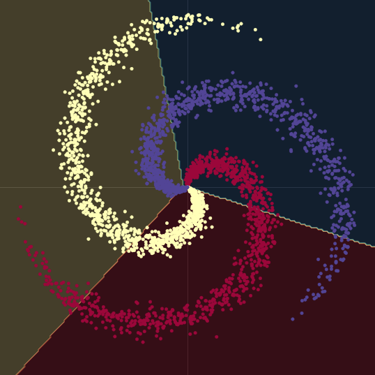
Fig. 9 Linear decision boundaries.

When we go from a linear model to one with two nn.linear() modules and a nn.ReLU() between them, the accuracy goes up to $95\%$. This is because the boundaries become non-linear and adapt much better to the spiral form of the data, as it can be seen in Fig. 10.

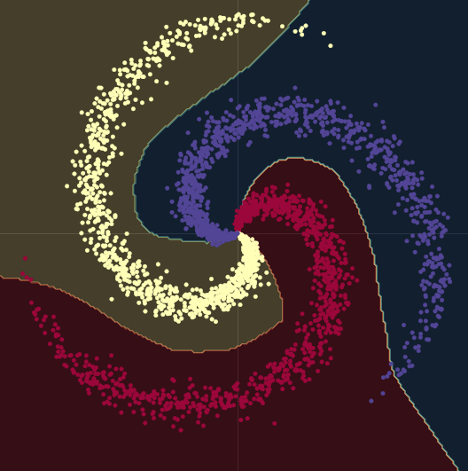
Fig. 10 Non-linear decision boundaries.

An example of a regression problem which can’t be solved correctly with a linear regression, but is easily solved with the same neural network structure can be seen in this notebook and Fig. 11, which shows 10 different networks, where 5 have a nn.ReLU() link function and 5 have a nn.Tanh(). The former is a piecewise linear function, whereas the latter is a continuous and smooth regression.

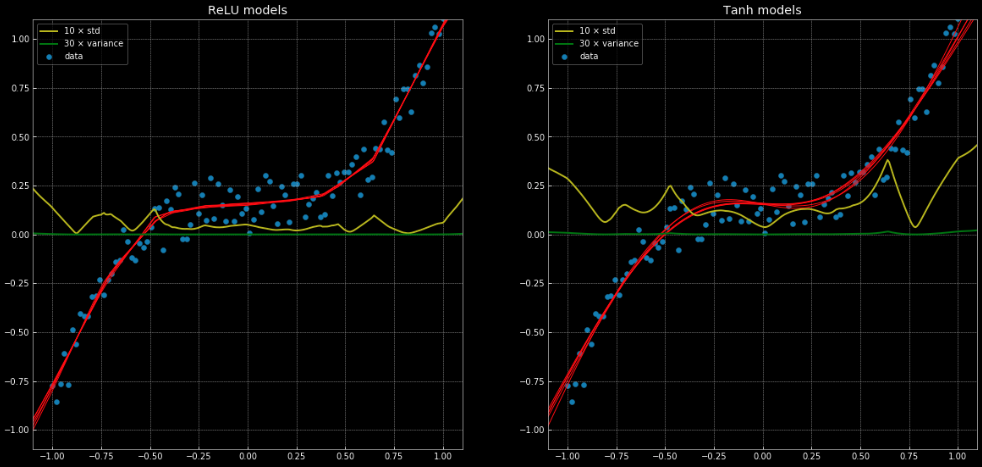
Fig. 11: 10 Neural networks, along with their variance and standard deviation.
Left: Five ReLU networks. Right: Five tanh networks.

The yellow and green lines show the standard deviation and variance for the networks. Using these is useful for something similar to a “confidence interval” – since the functions give a single prediction per output. Using ensemble variance prediction allows us to estimate the uncertainty with which the prediction is being made. The importance of this can be seen in Fig. 12, where we extend the decision functions outside the training interval and these tend towards $+\infty, -\infty$.

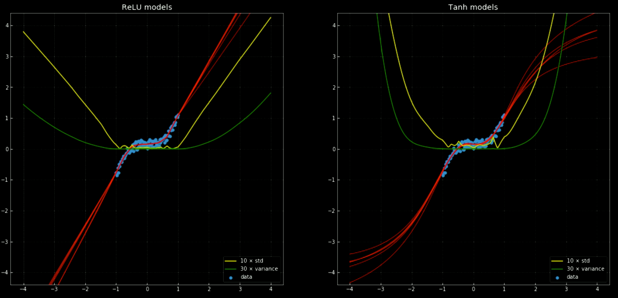
Fig. 12 Neural networks, with mean and standard deviation, outside training interval.
Left: Five ReLU networks. Right: Five tanh networks.

To train any Neural Network using PyTorch, you need 5 fundamental steps in the training loop:

1. output = model(input) is the model’s forward pass, which takes the input and generates the output.
2. J = loss(output, target <or> label) takes the model’s output and calculates the training loss with respect to the true target or label.
3. model.zero_grad() cleans up the gradient calculations, so that they are not accumulated for the next pass.
4. J.backward() does back-propagation and accumulation: It computes $\nabla_\texttt{x} J$ for every variable $\texttt{x}$ for which we have specified requires_grad=True. These are accumulated into the gradient of each variable: $\texttt{x.grad} \gets \texttt{x.grad} + \nabla_\texttt{x} J$.
5. optimiser.step() takes a step in gradient descent: $\vartheta \gets \vartheta - \eta\, \nabla_\vartheta J$.

When training a NN, it is very likely that you need these 5 steps in the order they were presented.

---

4 Feb 2020