Introduction to Gradient Descent and Backpropagation Algorithm

Gradient Descent optimization algorithm

Parametrised models

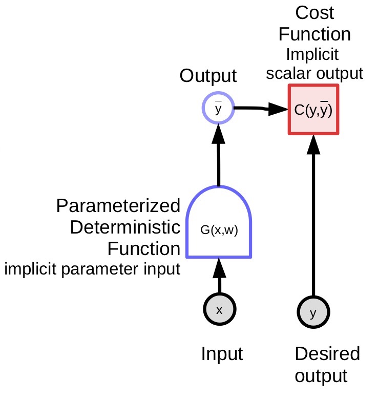
Parametrised models are simply functions that depend on inputs and trainable parameters. There is no fundamental difference between the two, except that trainable parameters are shared across training samples whereas the input varies from sample to sample. In most deep learning frameworks, parameters are implicit, that is, they aren’t passed when the function is called. They are ‘saved inside the function’, so to speak, at least in the object-oriented versions of models.

The parametrised model (function) takes in an input, has a parameter vector and produces an output. In supervised learning, this output goes into the cost function ($C(y,\bar{y}$)), which compares the true output (${y}$) with the model output ($\bar{y}$). The computation graph for this model is shown in Figure 1.

Figure 1: Computation Graph representation for a Parametrised Model

Examples of parametrised functions -

• Linear Model - Weighted Sum of Components of the Input Vector :

  \[\bar{y} = \sum_i w_i x_i, C(y,\bar{y}) = \Vert y - \bar{y}\Vert^2\]

• Nearest Neighbour - There is an input $\vect{x}$ and a weight matrix $\matr{W}$ with each row of the matrix indexed by $k$. The output is the value of $k$ that corresponds to the row of $\matr{W}$ that is closest to $\vect{x}$:

  \[\bar{y} = \underset{k}{\arg\min} \Vert x - w_{k,.} \Vert^2\]

  Parameterized models could also involve complicated functions.

Block diagram notations for computation graphs

• Variables (tensor, scalar, continuous, discrete)
  • is an observed input to the system
  • is a computed variable which is produced by a deterministic function

• Deterministic functions

  

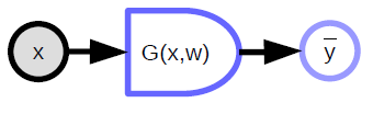
  • Takes in multiple inputs and can produce multiple outputs
  • It has an implicit parameter variable (${w}$)
  • The rounded side indicates the direction in which it is easy to compute. In the above diagram, it is easier to compute ${\bar{y}}$ from ${x}$ than the other way around

• Scalar-valued function

  

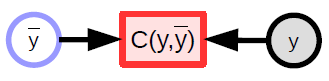
  • Used to represent cost functions
  • Has an implicit scalar output
  • Takes multiple inputs and outputs a single value (usually the distance between the inputs)

Loss functions

Loss function is a function that is minimized during training. There are two types of losses:

1) Per Sample Loss -

2) Average Loss -

For any set of Samples

Average Loss over the Set $S$ is given by:

Figure 2: Computation graph for model with Average Loss

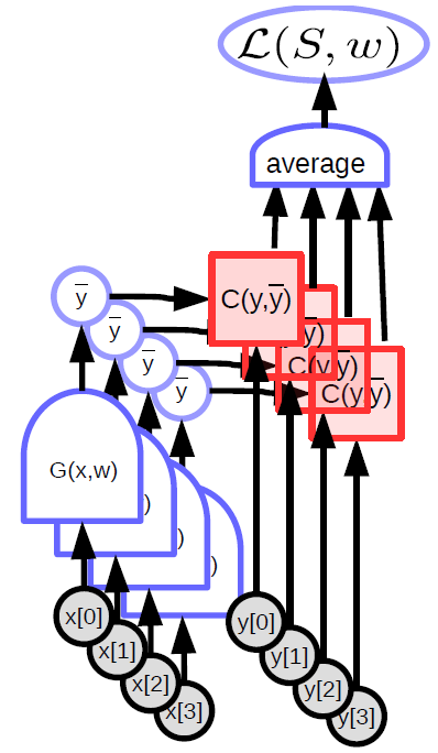In the standard Supervised Learning paradigm, the loss (per sample) is simply the output of the cost function. Machine Learning is mostly about optimizing functions (usually minimizing them). It could also involve finding Nash Equilibria between two functions like with GANs. This is done using Gradient Based Methods, though not necessarily Gradient Descent.

Gradient descent

A Gradient Based Method is a method/algorithm that finds the minima of a function, assuming that one can easily compute the gradient of that function. It assumes that the function is continuous and differentiable almost everywhere (it need not be differentiable everywhere).

Gradient Descent Intuition - Imagine being in a mountain in the middle of a foggy night. Since you want to go down to the village and have only limited vision, you look around your immediate vicinity to find the direction of steepest descent and take a step in that direction.

Different methods of Gradient Descent

• Full (batch) gradient descent update rule :

  \[w \leftarrow w - \eta \frac{\partial L(S,w)}{\partial w}\]

• For SGD (Stochastic Gradient Descent), the update rule becomes :

  • Pick a $p \in \lbrace 0, \cdots, P-1 \rbrace$, then update

    \[w \leftarrow w - \eta \frac{\partial L(x[p], y[p],w)}{\partial w}\]

Where ${w}$ represents the parameter to be optimized.

$\eta$ is a constant here but in more sophisticated algorithms, it could be a matrix.

If it is a positive semi-definite matrix, we’ll still move downhill but not necessarily in the direction of steepest descent. In fact the direction of steepest descent may not always be the direction we want to move in.

If the function is not differentiable, i.e, it has a hole or is staircase like or flat, where the gradient doesn’t give you any information, one has to resort to other methods - called 0-th Order Methods or Gradient-Free Methods. Deep Learning is all about Gradient Based Methods.

However, RL (Reinforcement Learning) involves Gradient Estimation without the explicit form for the gradient. An example is a robot learning to ride a bike where the robot falls every now and then. The objective function measures how long the bike stays up without falling. Unfortunately, there is no gradient for the objective function. The robot needs to try different things.

The RL cost function is not differentiable most of the time but the network that computes the output is gradient-based. This is the main difference between supervised learning and reinforcement learning. With the latter, the cost function $C$ is not differentiable. In fact it completely unknown. It just returns an output when inputs are fed to it, like a blackbox. This makes it highly inefficient and is one of the main drawbacks of RL - particularly when the parameter vector is high dimensional (which implies a huge solution space to search in, making it hard to find where to move).

A very popular technique in RL is Actor Critic Methods. A critic method basically consists of a second C module which is a known, trainable module. One is able to train the C module, which is differentiable, to approximate the cost function/reward function. The reward is a negative cost, more like a punishment. That’s a way of making the cost function differentiable, or at least approximating it by a differentiable function so that one can backpropagate.

Advantages of SGD and backpropagation for traditional neural nets

Advantages of Stochastic Gradient Descent (SGD)

In practice, we use stochastic gradient to compute the gradient of the objective function w.r.t the parameters. Instead of computing the full gradient of the objective function, which is the average of all samples, stochastic gradient just takes one sample, computes the loss, $L$, and the gradient of the loss w.r.t the parameters, and then takes one step in the negative gradient direction.

In the formula, $w$ is approached by $w$ minus the step-size, times the gradient of the per-sample loss function w.r.t the parameters for a given sample, ($x[p]$,$y[p]$).

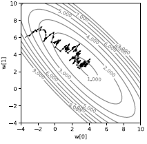
If we do this on a single sample, we will get a very noisy trajectory as shown in Figure 3. Instead of the loss going directly downhill, it’s stochastic. Every sample will pull the loss towards a different direction. It’s just the average that pulls us to the minimum of the average. Although it looks inefficient, it’s much faster than full batch gradient descent at least in the context of machine learning when the samples have some redundancy.

Figure 3: Stochastic Gradient Descent trajectory for per sample update

In practice, we use batches instead of doing stochastic gradient descent on a single sample. We compute the average of the gradient over a batch of samples, not a single sample, and then take one step. The only reason for doing this is that we can make more efficient use of the existing hardware (i.e. GPUs, multicore CPUs) if we use batches since it’s easier to parallelize. Batching is the simplest way to parallelize.

Traditional neural network

Traditional Neural Nets are basically interspersed layers of linear operations and point-wise non-linear operations. For linear operations, conceptually it is just a matrix-vector multiplication. We take the (input) vector multiplied by a matrix formed by the weights. The second type of operation is to take all the components of the weighted sums vector and pass it through some simple non-linearity (i.e. $\texttt{ReLU}(\cdot)$, $\tanh(\cdot)$, …).

Figure 4: Traditional Neural Network

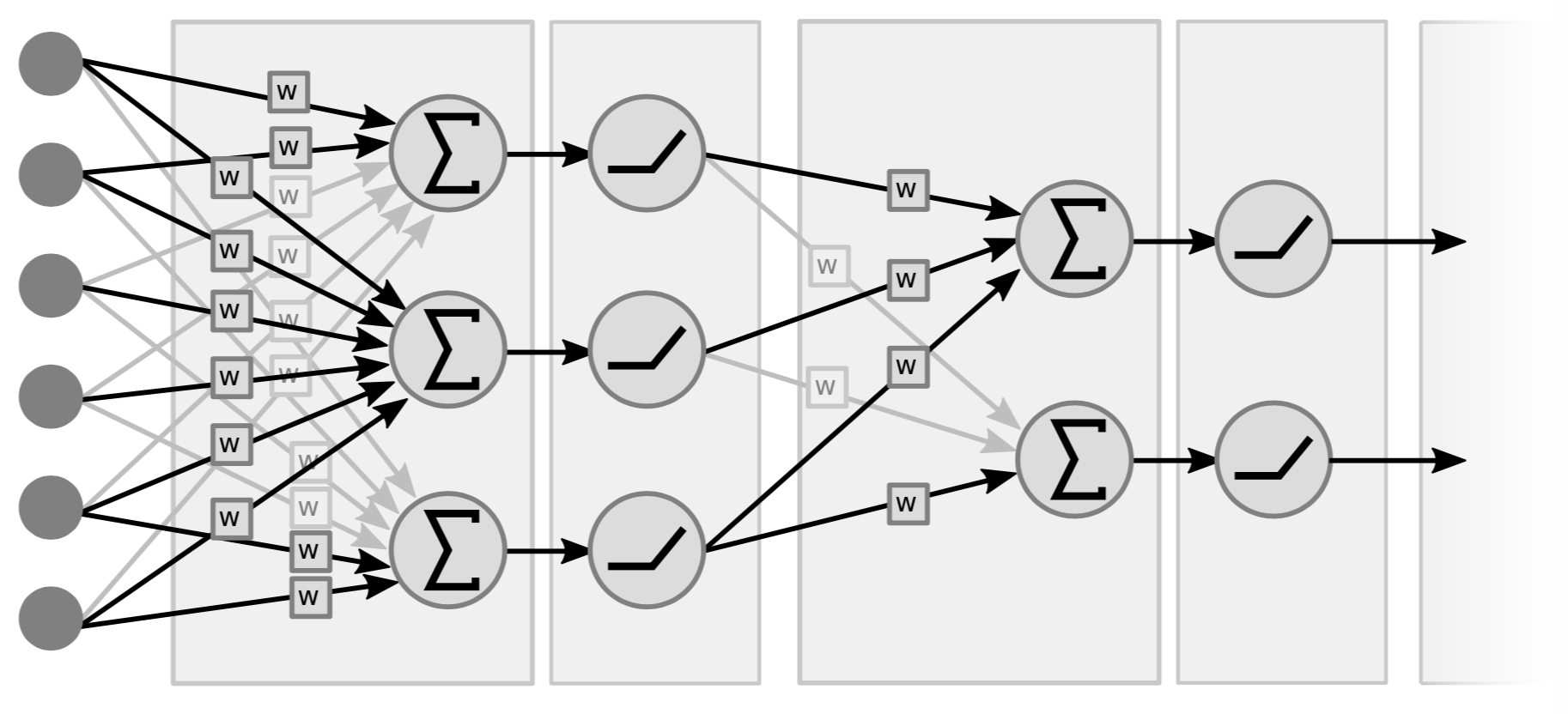Figure 4 is an example of a 2-layer network, because what matters are the pairs (i.e linear+non-linear). Some people call it a 3-layer network because they count the variables. Note that if there are no non-linearities in the middle, we may as well have a single layer because the product of two linear functions is a linear function.

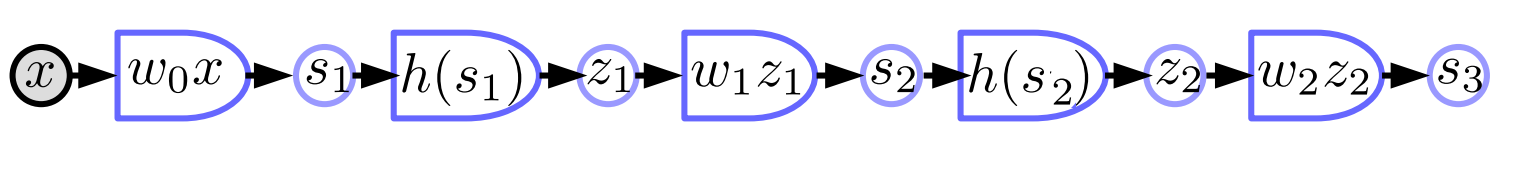
Figure 5 shows how the linear and non-linear functional blocks of the network stack:

Figure 5: Looking inside the linear and non-linear blocks

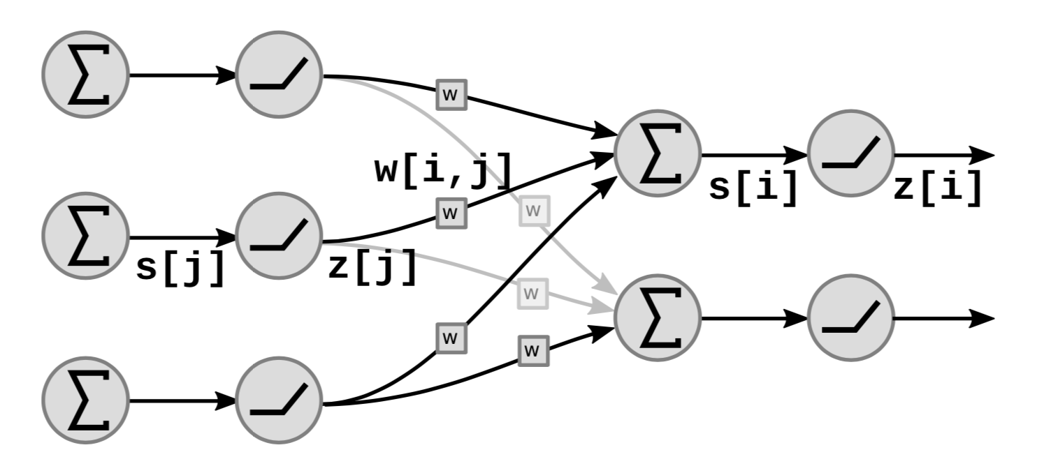In the graph, $s[i]$ is the weighted sum of unit ${i}$ which is computed as:

where $UP(i)$ denotes the predecessors of $i$ and $z[j]$ is the $j$th output from the previous layer.

The output $z[i]$ is computed as:

where $f$ is a non-linear function.

Backpropagation through a non-linear function

The first way to do backpropagation is to backpropagate through a non linear function. We take a particular non-linear function $h$ from the network and leave everything else in the blackbox.

Figure 6: Backpropagation through non-linear function

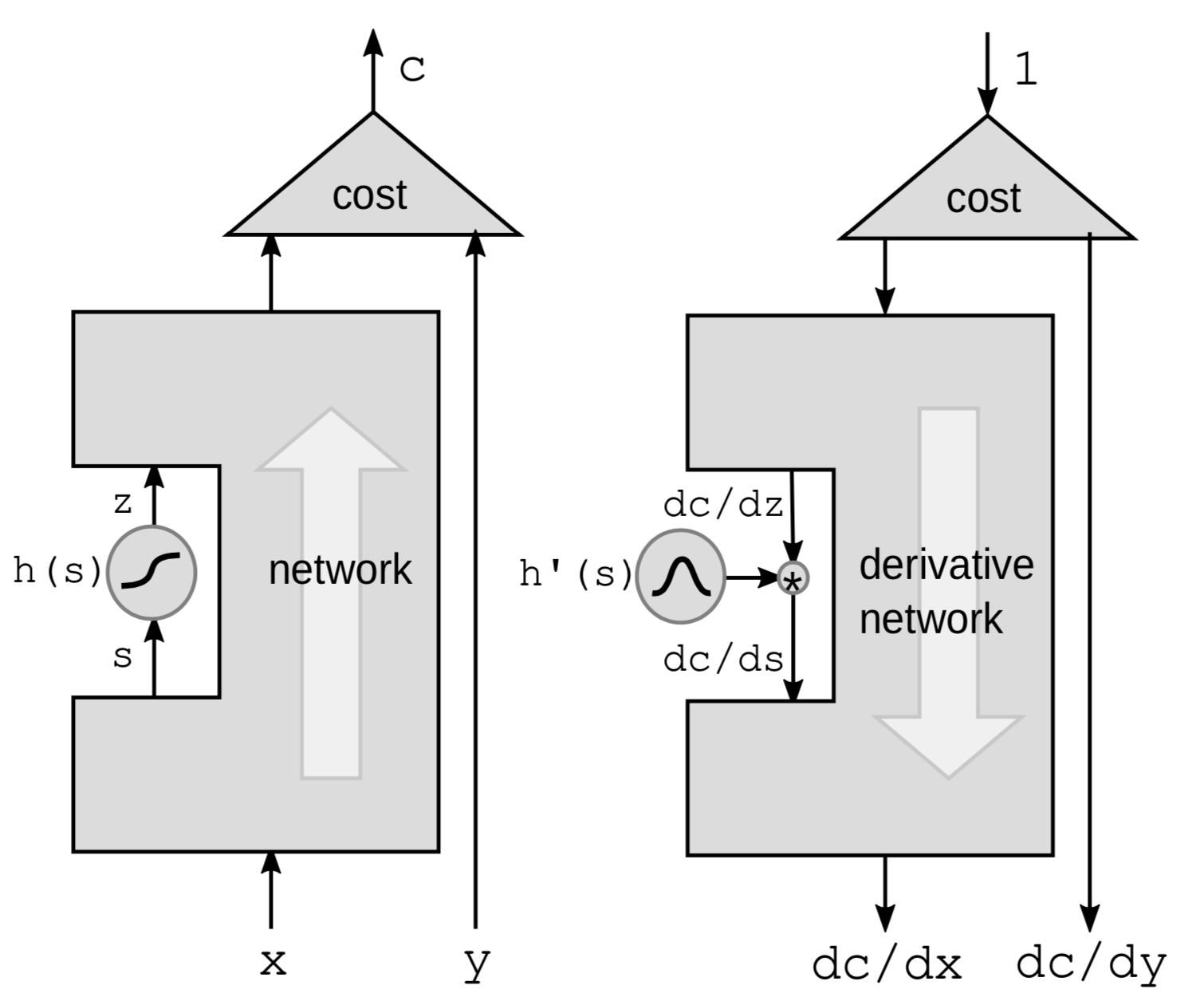We are going to use the chain rule to compute the gradients:

where $h’(s)$ is the derivative of $z$ w.r.t $s$ represented by $\frac{\mathrm{d}z}{\mathrm{d}s}$. To make the connection between derivatives clear, we rewrite the formula above as:

Hence if we have a chain of those functions in the network, we can backpropagate by multiplying by the derivatives of all the ${h}$ functions one after the other all the way back to the bottom.

It’s more intuitive to think of it in terms of perturbations. Perturbing $s$ by $\mathrm{d}s$ will perturb $z$ by:

This would in turn perturb $C$ by:

Once again, we end up with the same formula as the one shown above.

Backpropagation through a weighted sum

For a linear module, we do backpropagation through a weighted sum. Here we view the entire network as a blackbox except for 3 connections going from a ${z}$ variable to a bunch of $s$ variables.

Figure 7: Backpropagation through weighted sum

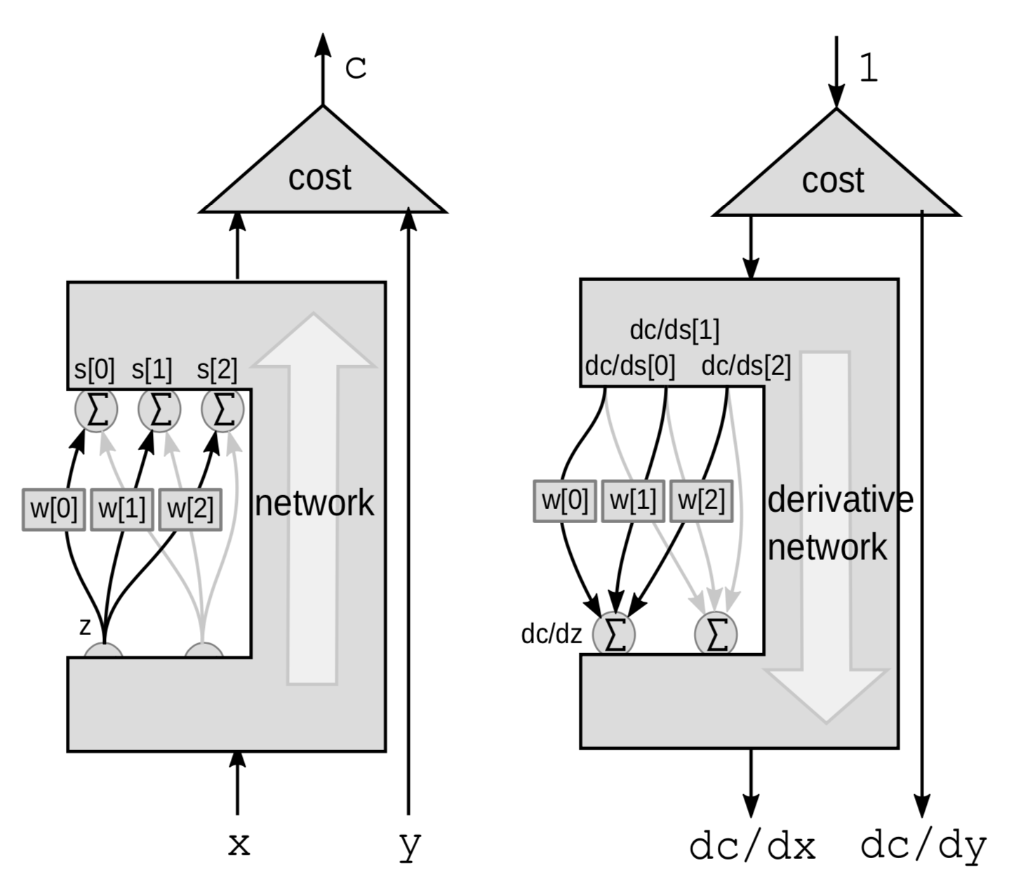This time the perturbation is a weighted sum. $Z$ influences several variables. Perturbing $z$ by $\mathrm{d}z$ will perturb $s[0]$, $s[1]$ and $s[2]$ by:

This will perturb $C$ by

Hence $C$ is going to vary by the sum of the 3 variations:

PyTorch implementation of neural network and a generalized backprop algorithm

Block diagram of a traditional neural net

• Linear blocks $s_{k+1}=w_kz_k$

• Non-linear blocks $z_k=h(s_k)$

  

$w_k$: matrix $z_k$: vector $h$: application of scalar ${h}$ function to every component. This is a 3-layer neural net with pairs of linear and non-linear functions, though most modern neural nets do not have such clear linear and non-linear separations and are more complex.

PyTorch implementation

import torch
from torch import nn
image = torch.randn(3, 10, 20)
d0 = image.nelement()

class mynet(nn.Module):
    def __init__(self, d0, d1, d2, d3):
        super().__init__()
        self.m0 = nn.Linear(d0, d1)
        self.m1 = nn.Linear(d1, d2)
        self.m2 = nn.Linear(d2, d3)

    def forward(self,x):
        z0 = x.view(-1)  # flatten input tensor
        s1 = self.m0(z0)
        z1 = torch.relu(s1)
        s2 = self.m1(z1)
        z2 = torch.relu(s2)
        s3 = self.m2(z2)
        return s3
model = mynet(d0, 60, 40, 10)
out = model(image)

• We can implement neural nets with object oriented classes in PyTorch. First we define a class for the neural net and initialize linear layers in the constructor using predefined nn.Linear class. Linear layers have to be separate objects because each of them contains a parameter vector. The nn.Linear class also adds the bias vector implicitly. Then we define a forward function on how to compute outputs with $\text{torch.relu}$ function as the nonlinear activation. We don’t have to initialize separate relu functions because they don’t have parameters.

• We do not need to compute the gradient ourselves since PyTorch knows how to back propagate and calculate the gradients given the forward function.

Backprop through a functional module

We now present a more generalized form of backpropagation.

Figure 8: Backpropagation through a functional module

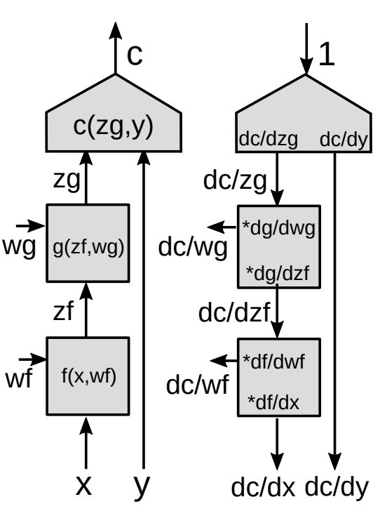• Using chain rule for vector functions

  \[z_g : [d_g\times 1]\] \[z_f:[d_f\times 1]\] \[\frac{\partial c}{\partial{z_f}}=\frac{\partial c}{\partial{z_g}}\frac{\partial {z_g}}{\partial{z_f}}\] \[[1\times d_f]= [1\times d_g]\times[d_g\times d_f]\]

  This is the basic formula for $\frac{\partial c}{\partial{z_f}}$ using the chain rule. Note that the gradient of a scalar function with respect to a vector is a vector of the same size as the vector with respect to which you differentiate. In order to make the notations consistent, it is a row vector instead of a column vector.

• Jacobian matrix

  \[\left(\frac{\partial{z_g}}{\partial {z_f}}\right)_{ij}=\frac{(\partial {z_g})_i}{(\partial {z_f})_j}\]

  We need $\frac{\partial {z_g}}{\partial {z_f}}$ (Jacobian matrix entries) to compute the gradient of the cost function with respect to $z_f$ given gradient of the cost function with respect to $z_g$. Each entry $ij$ is equal to the partial derivative of the $i$th component of the output vector with respect to the $j$th component of the input vector.

  If we have a cascade of modules, we keep multiplying the Jacobian matrices of all the modules going down and we get the gradients w.r.t all the internal variables.

Backprop through a multi-stage graph

Consider a stack of many modules in a neural network as shown in Figure 9.

Figure 9: Backprop through multi-stage graph

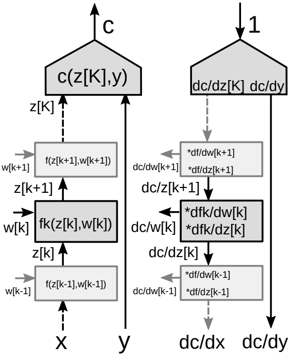For the backprop algorithm, we need two sets of gradients - one with respect to the states (each module of the network) and one with respect to the weights (all the parameters in a particular module). So we have two Jacobian matrices associated with each module. We can again use chain rule for backprop.

• Using chain rule for vector functions

  \[\frac{\partial c}{\partial {z_k}}=\frac{\partial c}{\partial {z_{k+1}}}\frac{\partial {z_{k+1}}}{\partial {z_k}}=\frac{\partial c}{\partial {z_{k+1}}}\frac{\partial f_k(z_k,w_k)}{\partial {z_k}}\] \[\frac{\partial c}{\partial {w_k}}=\frac{\partial c}{\partial {z_{k+1}}}\frac{\partial {z_{k+1}}}{\partial {w_k}}=\frac{\partial c}{\partial {z_{k+1}}}\frac{\partial f_k(z_k,w_k)}{\partial {w_k}}\]

• Two Jacobian matrices for the module

  • One with respect to $z[k]$
  • One with respect to $w[k]$