Graph Convolutional Networks I

🎙️ Xavier Bresson

Traditional ConvNets

ConvNets are powerful architectures to solve high-dimensional learning problems.

What is the Curse of Dimensionality?

Consider an image of 1024 x 1024 pixels. This image can be seen as a point in the space for 1,000,000 dimensions. Using 10 samples per dimension generates ${10}^{1,000,000}$ images, which is extremely high. ConvNets are extremely powerful to extract best representation of high-dimensional image data, such as the one given in the example.

• dim(image) = 1024 x 1024 = ${10}^{6}$
• For N = 10 samples/dim –> ${10}^{1,000,000}$ points

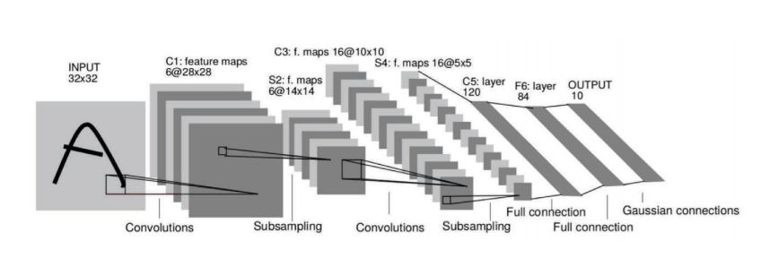
Fig. 1: ConvNets extract representation of high-dimensional image data.

Main assumptions about ConvNets:

1. Data (images, videos, speech) is compositional.

It is formed of patterns that are:

• Local A neuron in the neural network is only connected to the adjacent layers, but not to all layers in the network. We call this the local reception field assumption.
• Stationary We have some patterns that are similar and are shared across our image domain. For example, the yellow bedsheet in the middle image of figure 2.
• Hierarchical Low level features will be combined to form medium level features. Subsequently, these medium level features will combined to progressively form higher and higher level features. For example, a visual representation.

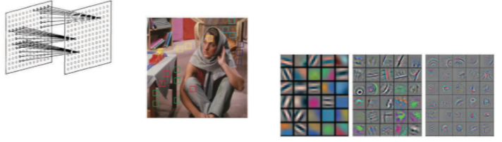
Fig. 2: Data is compositional.

2. ConvNets leverage the compositionality structure.

They extract compositional features and feed them to classifier, recommender, etc.

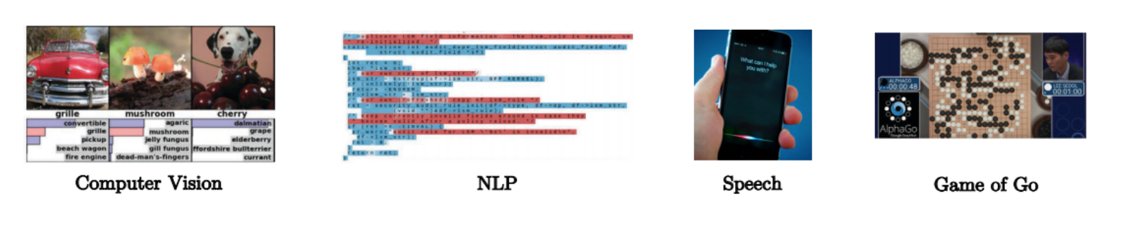
Fig. 3: ConvNets leverage the compositionality structure.

Graph Domain

Data Domain

• Images, volumes, videos lie on 2D, 3D, 2D+1 Euclidean domains (grids). Each pixel is represented by a vector of red, green, and blue values.

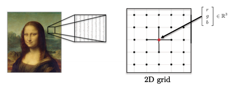
Fig. 4: Images have multiple dimensions.

• Sentences, words, speech lie on 1D Euclidean domain. For example, each character can be represented by an integer.

  
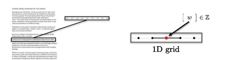
  Fig. 5: Sequences have single dimension.

• These domains have strong regular spatial structures, which allows all ConvNets operations to be fast and mathematically well defined.

  
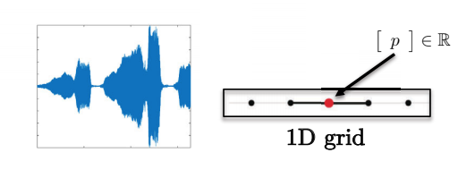
  Fig. 6: Speech data has 1D grid.

Graph Domain

Motivational Examples of graph domains

Let’s consider a social network. The social network is best captured by a graph representation since pair-wise connection between two users do not form a grid. Nodes of the graph represents users, whereas the edges between two nodes represent connection between two nodes (users). Each user has a three-dimensional feature matrix containing such as messages, images, and videos.

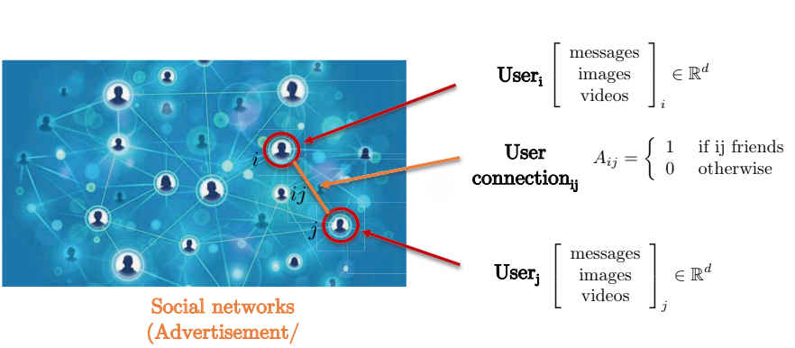
Fig. 7: Social networks by graph representation.

The connection between the structure and function of the brain to predict neural genetic diseases offers a motivational example to consider. As can be seen below, the brain is composed of several Region of Interest(s) (ROI). These ROIs is only locally connected to some surrounding regions of interests. Adjacency matrix represents the degree of strengths between different regions of interest.

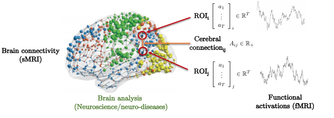
Fig. 8: Brain connectivity by graph representation.

Quantum Chemistry also offers an interesting representation of graphical domain. Each atom is represented by a node in graph and is connected to other atoms through bonds using edges. Each of these molecules/atoms have different features, such as the associated charge, bond type etc.

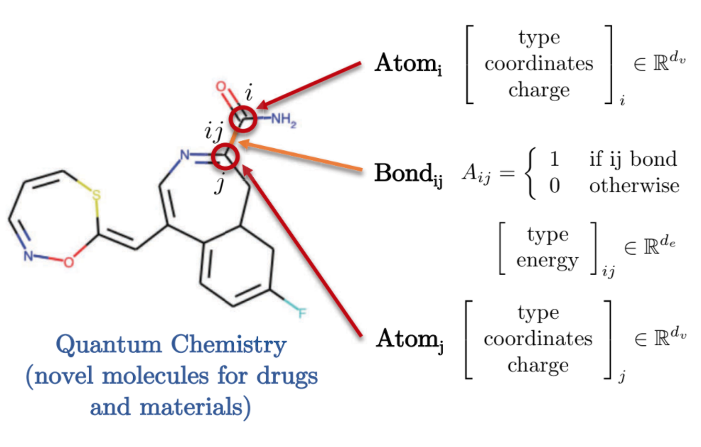
Fig. 9: Quantum chemistry by graph representation.

Graph Definition and Characteristics

• Graph G is defined by:
  • Vertices V
  • Edges E
  • Adjacency matrix A
• Graph features:
  • Node features: $h_{i}$, $h_{j}$ (atom type)
  • Edge features: $e_{ij}$ (bond type)
  • Graph features: g (molecule energy)

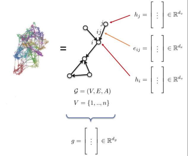
Fig. 10: Graph.

Convolution of Traditional ConvNets

Convolution

We abstractly define convolution as:

\(h^{\ell+l} = w^\ell * h^\ell,\) where $h^{\ell+1}$ is $n_1\times n_2\times d$-dimensional, $w^\ell$ is $3\times 3\times d$-dimensional, and $h^\ell$ is $n_1\times n_2\times d$-dimensional. For example, $n_1$ and $n_2$ could be the number of pixels in the $x$ and $y$ directions of an image, respectively, and $d$ is the dimensionality of each pixel (e.g., 3 for a colored image).
So, $h^{\ell+1}$ is a feature at the $(\ell+1)$-th hidden layer obtained by applying the convolution $w^\ell$ to a feature at the $\ell$-th layer.
Usually the kernel is small to represent a local reception field – $3\times 3$ in this case, or $5\times 5$, for example.
Note: we use padding to ensure the dimensions of $h^{\ell+1}$ are the same as those of $h^\ell$.\

For example, in this image, the kernel may be used to recognize lines.

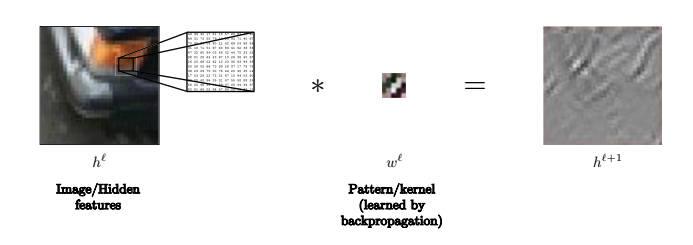
Fig. 11: Kernel can be used to recognize lines in images.

How do we define convolution?

More exactly, convolution is defined as follows:

\[h_i^{\ell+1} = w^\ell * h_i^\ell\] \[= \sum_{j\in\Omega}\langle w_j^\ell, h_{i-j}^\ell\rangle\] \[= \sum_{j\in\mathcal{N}_i} \langle w_j^\ell, h_{ij}^\ell\rangle\] \[=\sum_{j\in\mathcal{N}_i} \langle \Bigg[w_j^\ell\Bigg], \Bigg[h_{ij}\Bigg]\rangle\]

The above defines convolution as template matching.
We usually use $h_{i+j}$ instead of $h_{i-j}$, because the former is actually correlation, which is more like template matching.

However, it does not really matter if you use the first or second, because your kernel is just flipped, and this does not impact learning.

In the third line, we just write $h_{i+j}^\ell$ as $h_{ij}^\ell$.

The kernel is very small, so instead of summing over the whole image $\Omega$, as in the second line, we actually just sum over the neighborhood of cell $i$, $\mathcal{N}_i$, as denoted in the third line.

This makes it so that the complexity of convolution is $O(n)$, where $n$ is the number of pixels in the input image.

Convolution is exactly for each of the $n$ pixels, summing over inner products of vectors of dimension $d$ over $3\times 3$ grids.

The complexity is thus $n\cdot 3\cdot 3\cdot d$, which is $O(n)$; and moreover the computational can be done in parallel with GPUs at each of the $n$ pixels.

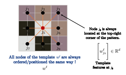
Fig. 12: Nodes are ordered in the same way.

If the graph you are convolving over is a grid, as in standard convolution over images in computer vision, then the nodes are ordered as in the above image. Therefore, $j_3$ will always be in the top right corner of the pattern.

So for all nodes $i$ in the image below, such as $i$ and $i’$, the node ordering of the kernel is always the same. For example, you always compare $j_3$ at the top right corner of the pattern with the top right corner of the image patch (what we convolve over for pixel $i$), as shown below. Mathematically speaking:

\[\langle\Bigg[w_{j_3}^\ell\Bigg], \Bigg[h_{ij_3}^\ell \Bigg]\rangle\]

and

\[\langle\Bigg[w_{j_3}^\ell\Bigg], \Bigg[h_{i'j_3}^\ell \Bigg]\rangle\]

are always for the top right corner between the template and the image patches.

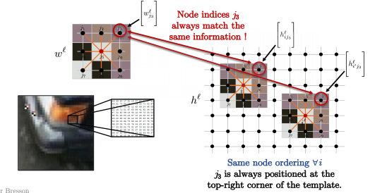
Fig. 13: Image patches match the templates.

Can we extend template matching for graphs?

We have a couple of issues:

1. First, in a graph, there is no ordering of the nodes.

So in the template shown below in the image, node $j_3$ has no specific position, but just an (arbitrary) index. So, when we try to match against nodes $i$ and $i’$ in the graph below, we do not know if $j_3$ is matching against the same nodes in both convolutions.
This is because there is no notion of the top right corner of the graph.
There is no notion of up, down, left right.
Thus, the template matchings actually have no meaning and we cannot use the definition of template matching directly, as above.

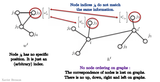
Fig. 14: No node ordering in a graph.

1. The second issue is that neighborhood sizes may be different.

So the template $w^\ell$ shown below has 4 nodes, but node $i$ has 7 nodes in its neighborhood. How can we compare these two?

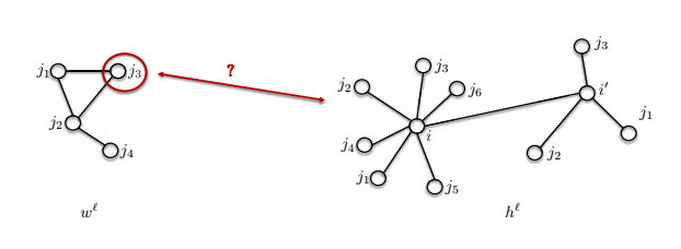
Fig. 15: Different neighborhood sizes in a graph.

Graph Convolution

We now use the Convolution Theorem to define convolution for graphs.

The Convolution Theorem states that the Fourier transform of the convolution of two functions is the pointwise product of their Fourier transforms:

\[\mathcal{F}(w*h) = \mathcal{F}(w) \odot \mathcal{F}(h) \implies w * h = \mathcal{F}^{-1}(\mathcal{F}(w)\odot\mathcal{F}(h))\]

In general, the Fourier transform has $O(n^2)$ complexity, but if the domain is a grid, then the complexity can be reduced to $O(n\log n)$ with FFT.

Can we extend the Convolution theorem to graphs?

This raises two questions:

1. How to define Fourier transforms for graphs?
2. How to compute fast spectral convolutions in $O(n)$ time for compact kernels (as in template matching)?

\[w *_{\mathcal{G}} h \stackrel{?}{=} \mathcal{F}^{-1}_{\mathcal{G}}(\mathcal{F}_{\mathcal{G}}(w)\odot\mathcal{F}_{\mathcal{G}}(h))\]

We are going to use these two design for graph neural networks: Template matching will be for spacial graph ConvNets and the Convolution theorem will be used for the spectral ConvNets.

Spectral Graph ConvNets

How to perform spectral convolution?

Step 1 : Graph Laplacian

This is the core operator in spectral graph theory.

Define

\[\begin{aligned} \mathcal{G}=(V, E, A) & \rightarrow \underset{n \times n}{\Delta}=\mathrm{I}-D^{-1 / 2} A D^{-1 / 2} \\ & \quad \text { where } \underset{n \times n} D=\operatorname{diag}\left(\sum_{j \neq i} A_{i j}\right) \end{aligned}\]

Note Matrix $A$ is the adjacency matrix, and the $\Delta$ is the Laplacian, which equals to the identity minus the adjacency matrix normalized by Matrix $D$. $D$ is a diagonal matrix, and each element on the diagonal is the degree of the node. This is called the normalized Laplacian, or Laplacian by default in this context.

The Laplacian is interpreted as the measurement of smoothness of graph, in other words, the difference between the local value $h_i$ and its neighborhood average value of $h_j$’s. $d_i$ on the formula below is the degree of node $i$, and $\mathcal{N}_{i}$ is the all the neighbors of node $i$.

\[(\Delta h)_{i}=h_{i}-\frac{1}{d_{i}} \sum_{j \in \mathcal{N}_{i}} A_{i j} h_{j}\]

The formula above is to apply Laplacian to a function $h$ on the node $i$, which is the value of $h_i$ minus the mean value over its neighboring nodes $h_j$’s. Basically, if the signal is very smooth, the Laplacian value is small, and vice versa.

Step 2 : Fourier Functions

The following is the eigen-decomposition of graph Laplacian,

\[\underset{n \times n}{\Delta}=\Phi^{T} \Lambda \Phi\]

The Laplacian is factorized into three matrices, $\Phi ^ T$, $\Lambda$, $\Phi$.

$\Phi$ is defined below, it contains column vectors, or Lap eigenvectors $\phi_1$ to $\phi_n$, each of size $n \times 1$, and those are also called Fourier functions. And Fourier functions form an orthonormal basis.

\[\begin{array}{l}\text { where } \underset{n \times n}{\Delta}\Phi=\left[\phi_{1}, \ldots, \phi_{n}\right]=\text { and } \Phi^{T} \Phi=\mathrm{I},\left\langle\phi_{k}, \phi_{k^{\prime}}\right\rangle=\delta_{k k^{\prime}} \\\end{array}\]

$\Lambda$ is a diagonal matrix with Laplacian eigenvalues, and on the diagonal are $\lambda_1$ to $\lambda_n$. And from the normalized applications, these values are typically among the range from $0$ to $2$. Those are also known as the Spectrum of a graph. See the formula below.

\[\begin{array}{c}\text { where } \underset{n \times n}\Lambda=\operatorname{diag}\left(\lambda_{1}, \ldots, \lambda_{n}\right) \text { and } 0 \leq \lambda_{1} \leq \ldots \leq \lambda_{n}=\lambda_{\max } \leq 2\end{array}\]

Below is an example of checking the eigenvalue decomposition. The Laplacian matrix $\Lambda$ is multiplied by an eigenvector $\phi_k$, the shape of the result is $n \times 1$, and the result is $\lambda_k \phi_k$.

\[\begin{array}{ll}\text { and } \underset{n \times 1}{\Delta \phi_{k}}=\lambda_{k} \phi_{k}, & k=1, \ldots, n \\ & \end{array}\]

The image below is the visualization of eigenvectors of 1D Euclidean Laplacian.

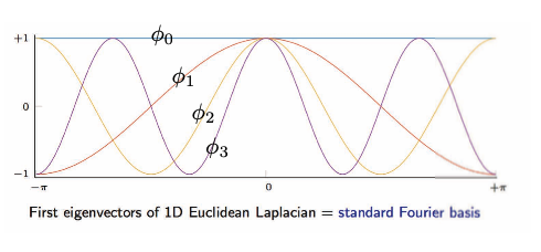
Fig. 16: Grid/Euclidean Domain: eigenvectors of 1D Euclidean Laplacian.

For graph domain, from the left to right, is the first, second, third, .. Fourier functions of a graph. For example, $\phi_1$ has oscillations of positive (red) and negative (blue) values, same for $\phi2$, $\phi3$. Those oscillations depend on the topology of a graph, which related to the geometry of graphs such as communities, hubs, etc, and it’s helpful for graph clustering. See below.

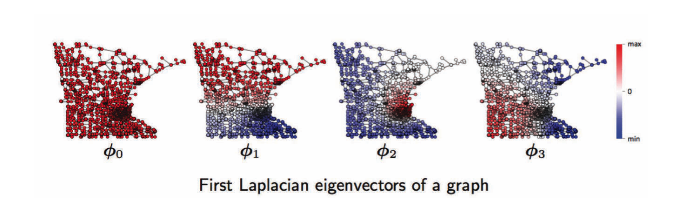
Fig. 17: Graph Domain: Fourier functions of a graph.

Step 3 : Fourier Transform

\[\begin{aligned} \underset{n \times 1} h &=\sum_{k=1}^{n} \underbrace{\left\langle\phi_{k}, h\right\rangle}_{\mathcal{F}(h)_{k}=\hat{h}_{k}=\phi_{k}^{T} h}\underset{n \times 1}{\phi_{k}} \\ &=\sum_{k=1}^{n} \hat{h}_{k} \phi_{k} \\ &=\underbrace{\Phi \hat{h}}_{ \mathcal{F}^{-1}(\hat{h}) } \end{aligned}\]

Fourier series: Decompose function $h$ with Fourier functions.

Take the function $h$ and projected on each Fourier function $\phi_k$, resulting in the coefficient of Fourier series of $k$, a scaler, and then multiplied by the function $\phi_k$.

The Fourier transform is basically projecting a function $h$ on the Fourier functions, and the result are the coefficients of the Fourier series.

Fourier Transform/ coefficients of Fourier Series

\[\begin{aligned} \underset{n \times 1}{\mathcal{F}(h)} &=\Phi^{T} h \\ &=\hat{h} \end{aligned}\]

Inverse Fourier Transform

\[\begin{aligned} \underset{n \times 1}{\mathcal{F}^{-1}(\hat{h})} &=\Phi \hat{h} \\ &=\Phi \Phi^{T} h=h \quad \text { as } \mathcal{F}^{-1} \circ \mathcal{F}=\Phi \Phi^{T}=\mathrm{I} \end{aligned}\]

Fourier transforms are linear operations, multiplying a matrix $\Phi^{T}$ with a vector $h$.

Step 4 : Convolution Theorem

Fourier transform of the convolution of two functions is the pointwise product of their Fourier transforms.

\[\begin{aligned} \underset{n \times 1} {w * h} &=\underbrace{\mathcal{F}^{-1}}_{\Phi}(\underbrace{\mathcal{F}(w)}_{\Phi^{T} w=\hat{w}} \odot \underbrace{\mathcal{F}(h)}_{\Phi^{T} h}) \\ &=\underset{n \times n}{\Phi}\left( \underset{n \times 1}{\hat{w}}\odot \underset{n \times 1}{\Phi^{T} h}\right) \\ &=\Phi\left(\underset{n \times n}{\hat{w}(\Lambda)} \underset{n \times 1}{\Phi^{T} h}\right) \\ &=\Phi \hat{w}(\Lambda) \Phi^{T} h \\ &=\hat{w}(\underbrace{\Phi \Lambda \Phi^{T}}_{\Delta}) h \\ &=\underset{n \times n}{\hat{w}(\Delta)} \underset{n \times1}h \\ & \end{aligned}\]

The example above is the convolution of $w$ and $h$, both of shape $n \times 1$, it equals the inverse of Fourier transform of pointwise product between Fourier transform of $w$ and of $h$. The formula above shows that it also equals to the matrix multiplication of $\hat{w}(\Delta)$ and $h$.

The convolution of two functions on the graph $h$ and $w$ is to take the spectrum function of $w$ and apply it to Laplacian and multiply it by $h$, and this is the definition of spectrum convolution. However, the computation complexity is $\mathrm{O}\left(n^{2}\right)$, while $n$ is the number of nodes in the graph.

Limitation

The spectral convolution against the graph domain is not shifting invariance, which means that if shifted, the shape of the function might also be changed, while in grid/euclidean domain does not.

Recommended book

Spectral graph theory, Fan Chung, (harmonic analysis, graph theory, combinatorial problems, optimization)

---

📝 Bilal Munawar, Alexander Bienstock, Can Cui, Shaoling Chen
27 Apr 2020