Problem Motivation, Linear Algebra, and Visualization

Resources

Please follow Alfredo Canziani on Twitter @alfcnz. Videos and textbooks with relevant details on linear algebra and singular value decomposition (SVD) can be found by searching Alfredo’s Twitter, for example type linear algebra (from:alfcnz) in the search box.

Transformations and motivation

As a motivating example, let us consider image classification. Suppose we take a picture with a 1 megapixel camera. This image will have about 1,000 pixels vertically and 1,000 pixels horizontally, and each pixel will have three colour dimensions for red, green, and blue (RGB). Each particular image can then be considered as one point in a 3 million-dimensional space. With such massive dimensionality, many interesting images we might want to classify – such as a dog vs. a cat – will essentially be in the same region of the space.

In order to effectively separate these images, we consider ways of transforming the data in order to move the points. Recall that in 2-D space, a linear transformation is the same as matrix multiplication. For example, the following are linear transformations:

• Rotation (when the matrix is orthonormal).
• Scaling (when the matrix is diagonal).
• Reflection (when the determinant is negative).
• Shearing.

Note that translation alone is not linear since 0 will not always be mapped to 0, but it is an affine transformation. Returning to our image example, we can transform the data points by translating such that the points are clustered around 0 and scaling with a diagonal matrix such that we “zoom in” to that region. Finally, we can do classification by finding lines across the space which separate the different points into their respective classes. In other words, the idea is to use linear and nonlinear transformations to map the points into a space such that they are linearly separable. This idea will be made more concrete in the following sections.

Data visualization - separating points by colour using a network

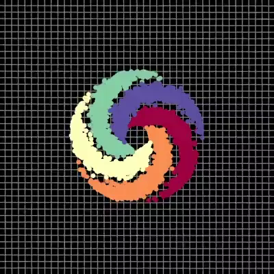
In our visualization, we have five branches of a spiral, with each branch corresponding to a different colour. The points live in a two dimensional plane and can be represented as a tuple; the colour represents a third dimension which can be thought of as the different classes for each of the points. We then use the network to separate each of the points by colour.

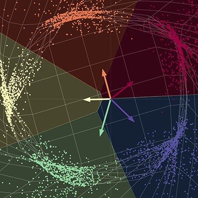(a) Input points, pre-network	(b) Output points, post-network

The network "stretches" the space fabric in order to separate each of the points into different subspaces. At convergence, the network separates each of the colours into different subspaces of the final manifold. In other words, each of the colours in this new space will be linearly separable using a one vs. all regression. The vectors in the diagram can be represented by a five by two matrix; this matrix can be multiplied to each point to return scores for each of the five colours. Each of the points can then be classified by colour using their respective scores. Here, the output dimension is five, one for each of the colours, and the input dimension is two, one for the x and y coordinates of each of the points. To recap, this network basically takes the space fabric and performs a space transformation parametrised by several matrices and then by non-linearities.

Network architecture

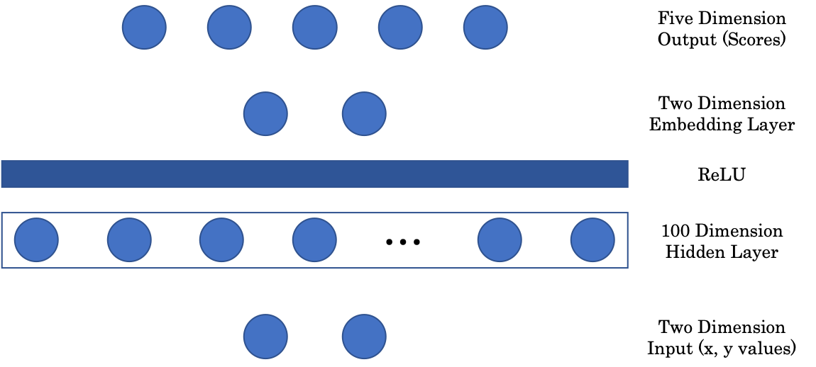
Figure 2: Network Architecture

The first matrix maps the two dimensional input to a 100 dimensional intermediate hidden layer. We then have a non-linear layer, ReLU or Rectified Linear Unit, which is simply positive part $(\cdot)^+$ function. Next, to display our image in a graphical representation, we include an embedding layer that maps the 100 dimensional hidden layer input to a two-dimensional output. Lastly, the embedding layer is projected to the final, five-dimensional layer of the network, representing a score for each colour.

Random projections - Jupyter Notebook

The Jupyter Notebook can be found here. In order to run the notebook, make sure you have the pDL environment installed as specified in README.md.

PyTorch device

PyTorch can run on both the CPU and GPU of a computer. The CPU is useful for sequential tasks, while the GPU is useful for parallel tasks. Before executing on our desired device, we first have to make sure our tensors and models are transferred to the device’s memory. This can be done with the following two lines of code:

device = torch.device("cuda:0" if torch.cuda.is_available() else "cpu")
X = torch.randn(n_points, 2).to(device)

The first line creates a variable, called device, that is assigned to the GPU if one is available; otherwise, it defaults to the CPU. In the next line, a tensor is created and sent to the device’s memory by calling .to(device).

Jupyter Notebook tip

To see the documentation for a function in a notebook cell, use Shift + Tab.

Visualizing linear transformations

Recall that a linear transformation can be represented as a matrix. Using singular value decomposition, we can decompose this matrix into three component matrices, each representing a different linear transformation.

In eq. (1), matrices $U$ and $V^\top$ are orthogonal and represent rotation and reflection transformations. The middle matrix is diagonal and represents a scaling transformation.

We visualize the linear transformations of several random matrices in Fig. 3. Note the effect of the singular values on the resulting transformations.

The matrices used were generated with Numpy; however, we can also use PyTorch’s nn.Linear class with bias = False to create linear transformations.

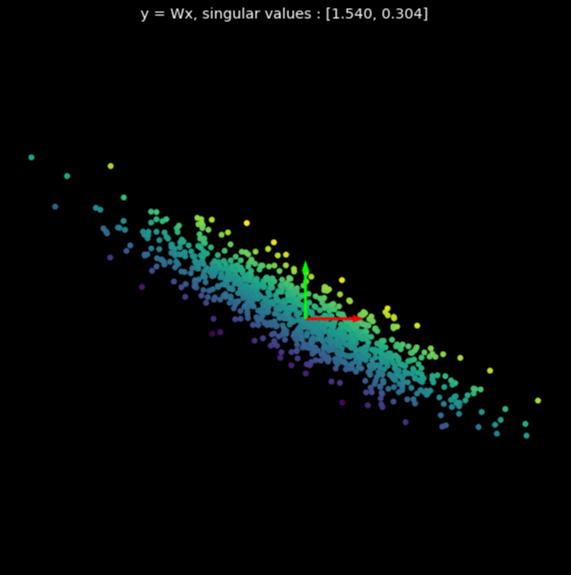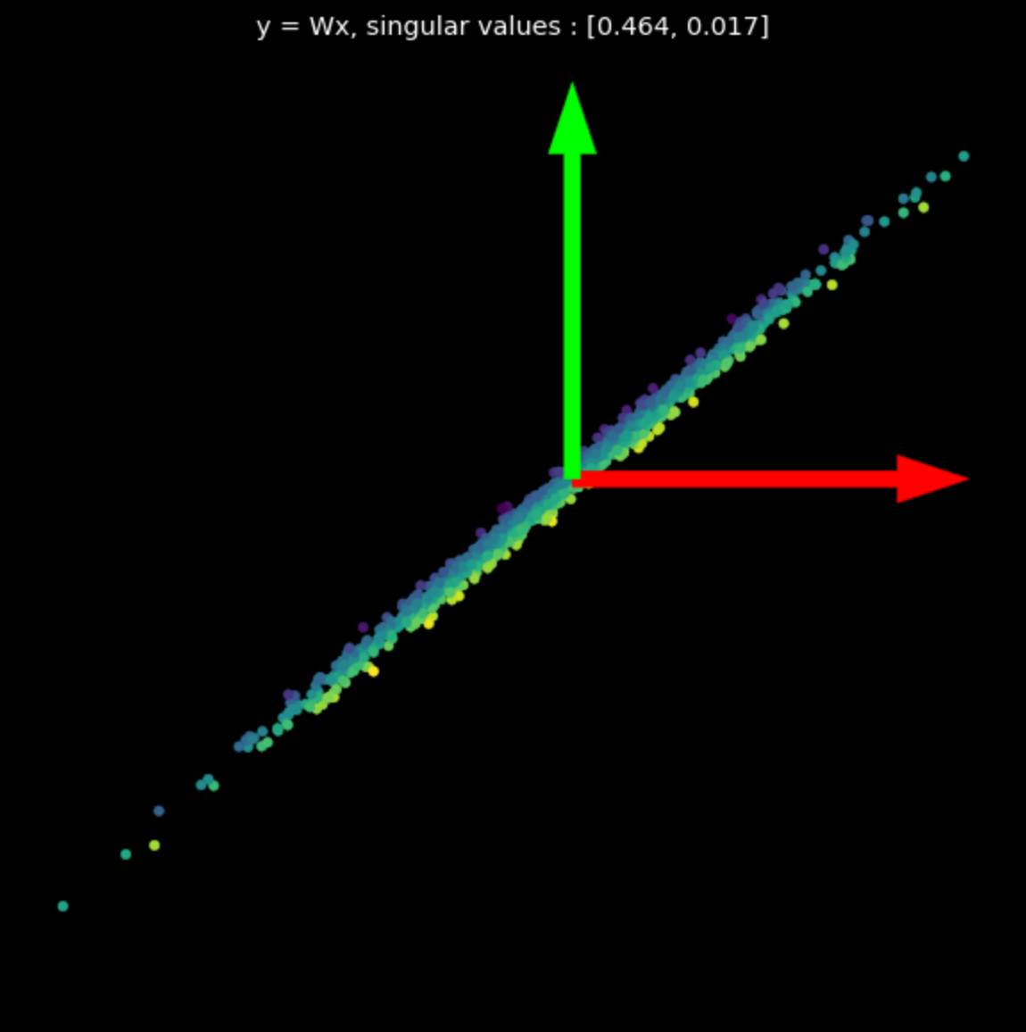(a) Original points	(b) $s_1$ = 1.540, $s_2$ = 0.304	(c) $s_1$ = 0.464, $s_2$ = 0.017

Non-linear transformations

Next, we visualize the following transformation:

Recall, the graph of $\tanh(\cdot)$ in Fig. 4.

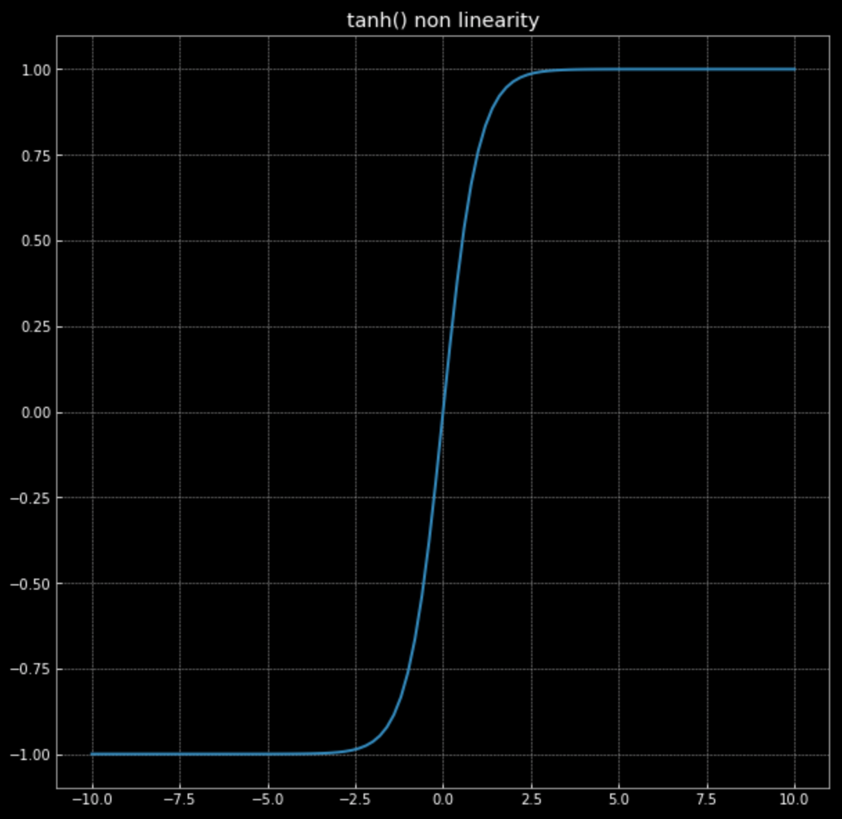
Figure 4: hyperbolic tangent non-linearity

The effect of this non-linearity is to bound points between $-1$ and $+1$, creating a square. As the value of $s$ in eq. (2) increases, more and more points are pushed to the edge of the square. This is shown in Fig. 5. By forcing more points to the edge, we spread them out more and can then attempt to classify them.

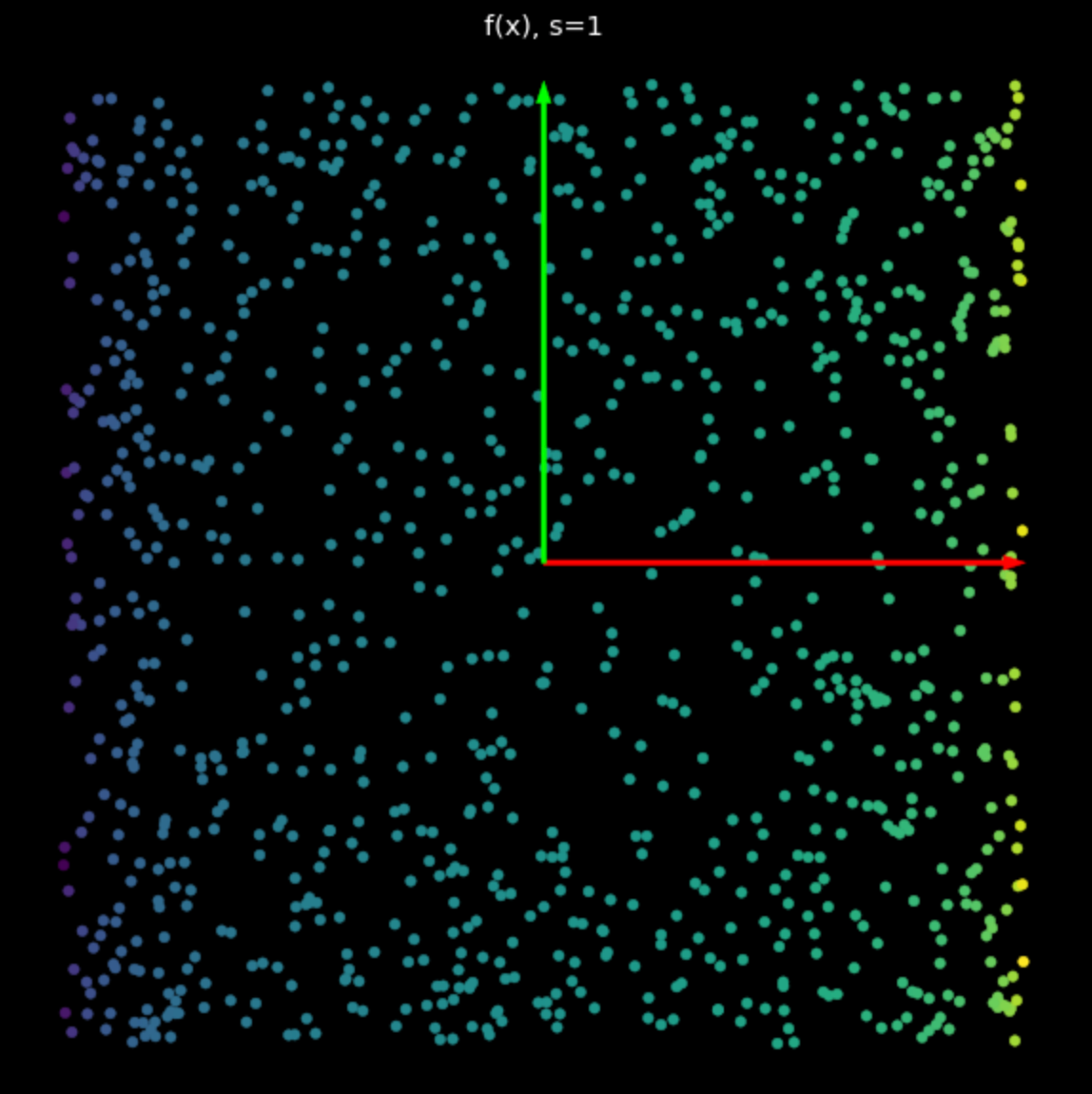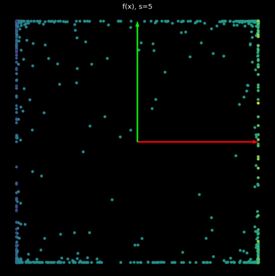(a) Non-linearity with $s=1$	(b) Nonlinearity with $s=5$

Random neural net

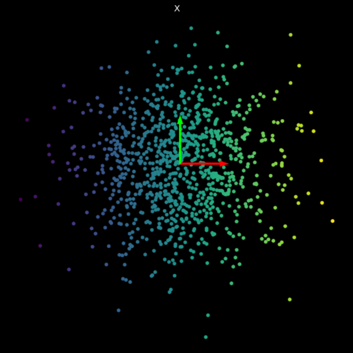
Lastly, we visualize the transformation performed by a simple, untrained neural network. The network consists of a linear layer, which performs an affine transformation, followed by a hyperbolic tangent non-linearity, and finally another linear layer. Examining the transformation in Fig. 6, we see that it is unlike the linear and non-linear transformations seen earlier. Going forward, we will see how to make these transformations performed by neural networks useful for our end goal of classification.

Figure 6: Transformation from an untrained neural network