Graphical Energy-based Methods
🎙️ Yann LeCunComparing losses
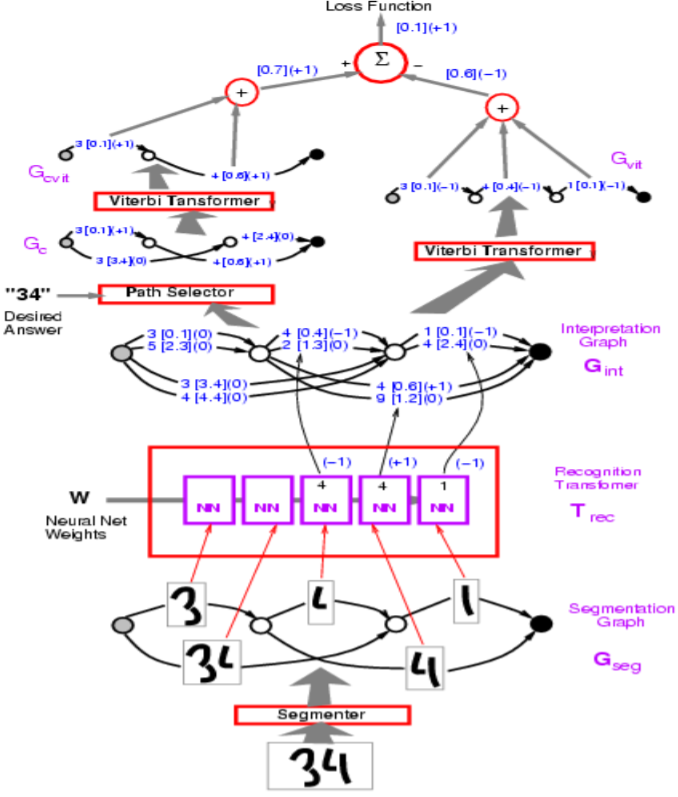
Figure 1: Network Architecture
In the figure above, incorrect paths have $-1$.
Professor LeCun starts with perceptron loss, which is used in the example of Graph Transformer Model in the figure above. The goal is to make energy of wrong answers large, and correct ones small.
In terms of implementation, you would represent the arcs in the visualization with a vector. Rather than a separate arc for each category, one vector contains both the categories and the score for each category.
Q: How is the segmentor implemented in the model above?
A: The segment is handcrafted heuristics. The model uses a handcrafted segment although there is a way to make it trainable end-to-end. This handcrafted approach was superseded by the sliding window approach for character recognition.
Overview of losses
| Loss Equation | Formula | Margin |
|---|---|---|
| Energy Loss | $\text{E}(\text{W}, \text{Y}^i, \text{X}^i)$ | None |
| Perceptron | $\text{E}(\text{W}, \text{Y}^i, \text{X}^i)-\min\limits_{\text{Y}\in\mathcal{Y}}\text{E}(\text{W}, \text{Y}, \text{X}^i)$ | 0 |
| Hinge | $\max\big(0, m + \text{E}(\text{W}, \text{Y}^i,\text{X}^i)-\text{E}(\text{W}, \overline{\text{Y}}^i,\text{X}^i)\big)$ | $m$ |
| Log | $\log\bigg(1+\exp\big(\text{E}(\text{W}, \text{Y}^i,\text{X}^i)-\text{E}(\text{W}, \overline{\text{Y}}^i,\text{X}^i)\big)\bigg)$ | >0 |
| LVQ2 | $\min\bigg(M, \max\big(0, \text{E}(\text{W}, \text{Y}^i,\text{X}^i)-\text{E}(\text{W}, \overline{\text{Y}}^i,\text{X}^i)\big)\bigg)$ | 0 |
| MCE | $\bigg(1+\exp\Big(-\big(\text{E}(\text{W}, \text{Y}^i,\text{X}^i)-\text{E}(\text{W}, \overline{\text{Y}}^i,\text{X}^i)\big)\Big)\bigg)^{-1}$ | >0 |
| Square-Square | $\text{E}(\text{W}, \text{Y}^i,\text{X}^i)^2-\bigg(\max\big(0, m - \text{E}(\text{W}, \overline{\text{Y}}^i,\text{X}^i)\big)\bigg)^2$ | $m$ |
| Square-Exp | $\text{E}(\text{W}, \text{Y}^i,\text{X}^i)^2 + \beta\exp\big(-\text{E}(\text{W}, \overline{\text{Y}}^i,\text{X}^i)\big)$ | >0 |
| NNL/MMI | $\text{E}(\text{W}, \text{Y}^i,\text{X}^i) + \frac{1}{\beta}\log\int_{y\in\mathcal{Y}}\exp\big(-\beta\text{E}(\text{W}, y,\text{X}^i)\big)$ | >0 |
| MEE | $1-\frac{\exp\big(-\beta E(W,Y^i,X^i)\big)}{\int_{y\in\mathcal{Y}}\exp\big(-\beta E(W,y,X^i)\big)}$ | >0 |
The perceptron loss seen in the table above does not have a margin, and thus the loss has a risk of collapsing.
- Hinge loss is taking the energy of the most offending answer, and the correct answer, and computing their difference. Intuitively, with a margin m, the hinge will only have loss of 0 when the correct energy is lower than the most offending energy by at least m.
- MCE loss is used in speech recognition, and looks similar to a sigmoid.
- NLL loss aims to make the energy of the correct answer small, and make the log component of the equation large.
Q: How may hinge be better than NLL loss?
A: Hinge is better than NLL because NLL will try to push the difference between the correct answer and other answers to infinity, whereas hinge only wants to make it larger than some value (the margin m).
Definition:
A decoder inputs a sequence of vectors that indicate the scores or energy of individual sounds or images, and picks out the best possible output.
Q: What are some examples of problems that can use decoders? A: Language modelling, machine translation, and sequence tagging.
Forward algorithm in Graph Transformer Networks
Graph composition
Graph composition allows us to combine two graphs. In this example we can see a language model lexicon being represented as a $trie$ (a graph) and a recognition graph which is produced by a neural network.
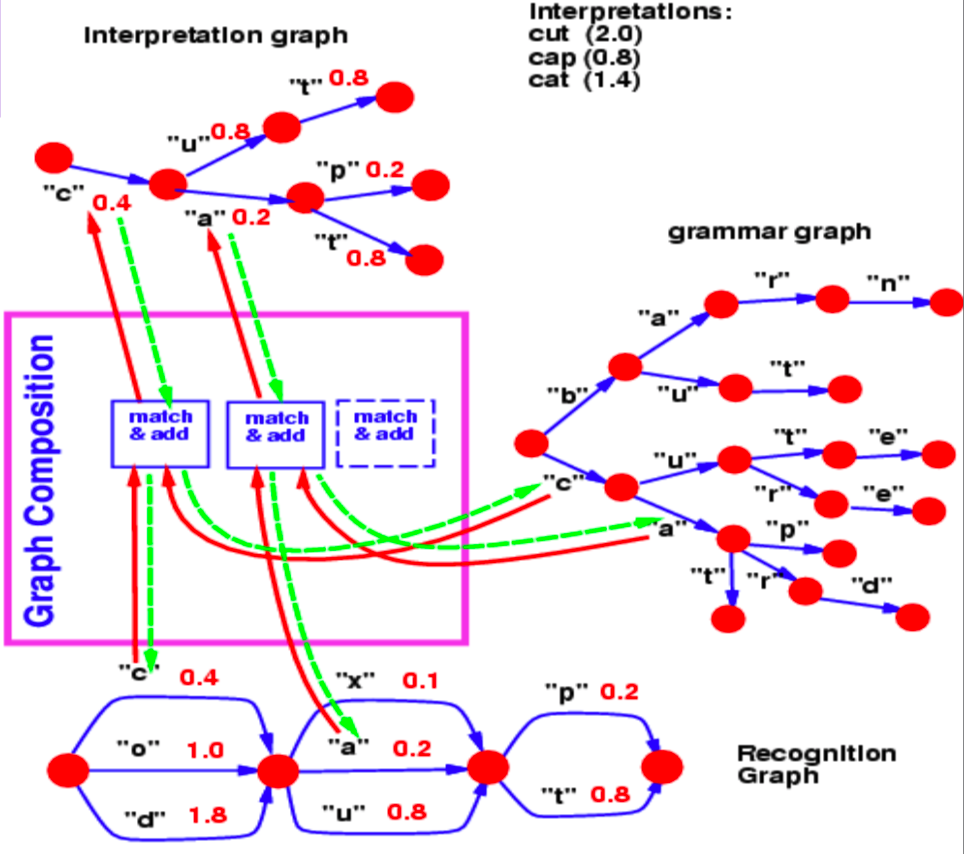
Figure 2: Graph Composition
The recognition graph specifies with different energy values (associated with each arc) how likely a character is at a particular step.
Now, for this example, the question we answer with a graph composition operation is, what is the best path in this recognition graph that also agrees with our lexicon?
The common hop from step 1 to step 2 between the recognition graph and the grammar is the character $c$, associated with energy 0.4. Hence, our interpretation graph contains just 1 arc between step 1 and 2 corresponding to $c$. Similarly, possible characters between step 2 and 3 are $x$, $u$ and $a$ in the recognition graph. Branches following $c$ in the grammar graph contain $u$ and $a$. So, the graph composition operation picks out arcs $u$ and $a$ to be present in the interpretation graph. It also associates the arc it copies from the recognition graph with their energy values.
If the grammar also contained energy values associated with arcs, the graph composition would have added the energy values or combined them using some other operator.
In a similar fashion, graph composition also allows us to combine two knowledge bases that are represented by neural networks. In the example discussed above, the grammar can essentially be represented as a neural network predicting the next character. The softmax output of the NN provides us with the transition probabilities to the next character from a given node.
As a side note, if the language model shown in this example is a neural network, we can backpropagate through the entire structure. This becomes an example of a differentiable program where we backpropagate through a program containing loops, if-conditions, recursions etc.
A check reader from mid-90s
The entire architecture of a check reader from the mid-90s is quite complex, but what we are primarily interested in, is the part starting from the character recogniser, which produces the recognition graph.
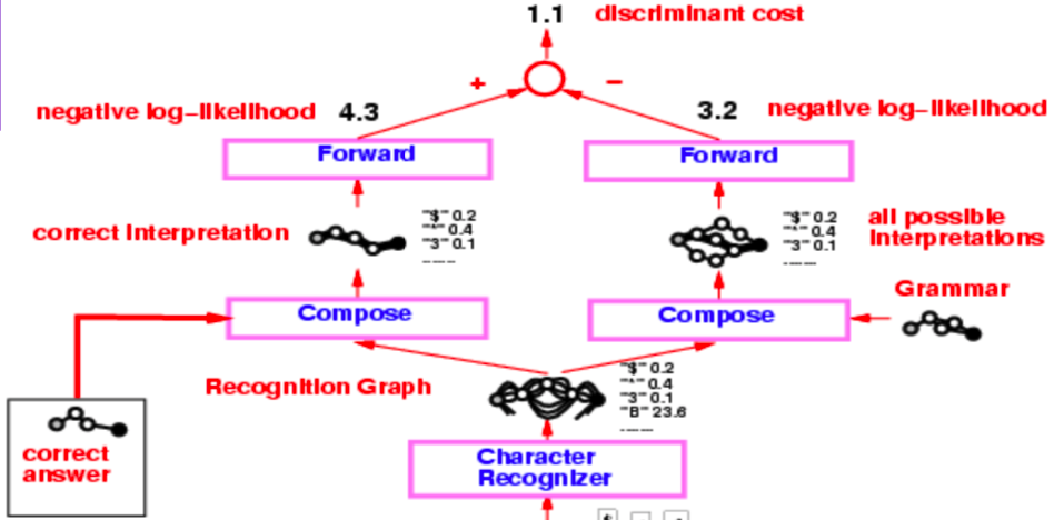
Figure 3: Check reader
This recognition graph undergoes two separate composition operations, one with the correct interpretation (or the ground truth) and second with the grammar which creates a graph of all possible interpretations.
The entire system is trained via the Negative Log-Likelihood loss function. The negative log-likelihood says that each path in the interpretation graph is a possible interpretation and sum of energies along that path is the energy of that interpretation.
Now, instead of using the Viterbi algorithm, we use the forward algorithm. The following sub-sections discuss the differences between the two approaches.
Viterbi algorithm
Viterbi algorithm is a dynamic programming algorithm that is used to find the most likely path (or the path with the minimum energy) in a given graph. It minimises the energy with respect to a latent variable z, where z represents the path we are taking in the graph.
\[F (x, y) = \min_{z} \; E(x, y, z)\]The forward algorithm
The forward algorithm, on the other hand, computes the log of sum of exponentials of the negative value of energies of all paths. This mouthful can be easily seen as a formula below:
\[F_{\beta} (x, y) = -\frac{1}{\beta} \; \log \; \sum_{z \, \in \, \text{paths}} \; \exp \, (- \beta \; E(x, y, z))\]This is marginalising over the latent variable z, which defines the paths in an interpretation graph. This approach computes this log sum exponential value over all possible paths to a particular node. This is like combining the cost of all possible paths in a soft-minimum way.
The forward algorithm is cheap to implement and does not cost more than Viterbi algorithm. Also, we can backpropagate through the forward algorithm node in the graph.
The working of the forward algorithm can be shown using the following example defined on an interpretation graph.
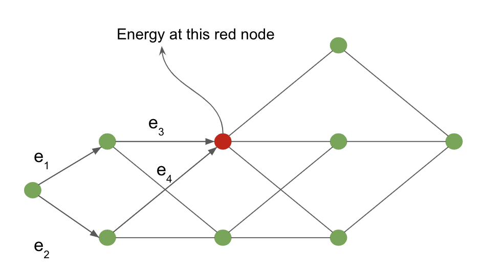
Figure 4: Interpretation graph
The cost from the input node to the red shaded node is computed by marginalising over all possible paths reaching the red node. The arrows entering the red node define these possible paths in our example.
For the red node, the value of energy at the node is given by:
\[-\frac{1}{\beta} \; \log \; [ \, \exp \, (- \, \beta (e_1 \, + \, e_3)) \; + \; \exp \, (- \, \beta (e_2 \, + \, e_4)) \, ]\]Neural network analogy of forward algorithm
The forward algorithm is a special case of the belief-propagation algorithm, when the underlying graph is a chain graph. This entire algorithm can be viewed as a feed-forward neural network where the function at each node is a log sum of exponentials and an addition term.
For each node in the interpretation graph, we maintain a variable $\alpha$.
\[\alpha_{i} = - \; \log \; \biggl[ \sum_{k \, \in \, \text{parent} \, (i)} \; \exp \, (- \, \beta \; (\alpha_k \, + \, e_{ki})) \biggl]\]where $e_{ki}$ is the energy of the link from node $k$ to node $i$.
$\alpha_i$ forms the activation of a node $i$ in this neural network and $e_{ki}$ is the weight between nodes $k$ and node $i$. This formulation is algebraically equivalent to the weighted sum operations of a regular neural network in the log domain.
We can backpropagate through the dynamic interpretation graph (since it changes from example to example) on which we apply the forward algorithm. We can compute the gradients of $F(x, y)$ computed at the last node of the graph w.r.t the $e_{ki}$ weights defining the edges of the interpretation graph.
Figure 5: Check reader
Returning back to the check reader example, we apply the forward algorithm on the two graph compositions and obtain the energy value at the last node using the log sum exponential formula. The difference between these energy values is the negative log-likelihood loss.
The value obtained from applying the forward algorithm on the graph composition between correct answer and recognition graph is the log sum exponential value of the correct answer. In contrast, log sum exponential value at the last node of the graph composition between recognition graph and grammar is the marginalised value over all possible valid interpretations.
Lagrangian formulation of backpropagation
For an input $x$ and target output $y$, we can formulate a network as a collection of functions, $f_k$ and weights, $w_k$ such that successive steps in the network output $z_k$ with $z_{k+1} = f_k(z_k, w_k)$. In a supervised setting, the goal of the network is to minimize $C(z_n, y)$, the cost of the $n^\mathrm{th}$ output of the network, with respect to the ground truth. This is equivalent to the problem of minimizing $C(z_n, y)$ with respect to the constraints $z_{k+1} = f_k(z_k, w_k)$ and $z_0 = x$.
The Lagrangian can be written: \(\mathcal{L}(x, y, \lambda_i, z_i, w_i) = C(z_n, y) + \sum\limits_{k=0}^{n-1} \lambda^T_{k+1}(z_{k+1} - f_k(z_k, w_k))\) where the $ \lambda $ terms denote Lagrange multipliers (see Paul’s online notes for a refresher if Calc 3 was a while ago).
To minimize $\mathcal{L}$, we need to set the partial derivatives of $\mathcal{L}$ with respect to each of its arguments to zero and solve.
- For $\lambda$, we simply recover the constraint: $\frac{\partial{\mathcal{L}}}{\partial \lambda_{k+1}} = 0 \rightarrow z_{k+1} = f_k(z_k, w_k)$.
- For $z_k$, $\frac{\partial \mathcal{L}}{\partial z_k} = 0 \rightarrow \lambda^T_k - \lambda^T_{k+1} \frac{\partial f_k(z_k, w)}{\partial z_k} \rightarrow \lambda_k = \frac{\partial f_k(z_k, w_k)^T}{\partial z_k}\lambda_{k+1}$, which is just the standard backpropagation formula.
This approach originated with Lagrange and Hamilton in the context of Classical Mechanics, where the minimization is over the energy of the system and the $\lambda$ terms denote physical constraints of the system, such as two balls being forced to stay at a fixed distance from each other by virtue of being attached by a metal bar, for example.
In a situation where we need to minimize the cost $C$ at every time step, $k$, the Lagrangian becomes \(\mathcal{L} = \sum_k \left(C_k(z_k, y_k) + \lambda^T_{k+1}(z_{k+1} - f_k(z_k, w_k)) \right)\).
Neural Ordinary Differential Equation
Using this formulation of backprop, we can now talk about a new class of models, Neural ODEs. These are basically recurrent networks where the state, $z$, at time $t$ is given by $ z_{t+\text{d}t} = z_t + f(z_t, W) dt $, where $ W$ represents some set of fixed parameters. This can also be expressed as an ordinary differential equation (no partial derivatives): $\frac{\text{d}z}{\text{d}t} = f(z_t, W)$.
Training such a network using the Lagrangian formulation is very straightforward. If we have a target, $y$, and want the state of the system to reach $y$ by time $T$, we simply establish the cost function as the distance between $z_T$ and $y$. Another goal of the network could be to find a stable state of the system, i.e. one that ceases to change after a certain point. Mathematically, this is equivalent to setting $\frac{\text{d}z}{\text{d}t} = f(y, W) = 0$. In general, finding a solution, $y$ to this equation is much easier than back propagation through time, because the network need not remember the gradient with respect to the whole sequence, and only has to minimize $f$ or $\lvert f \rvert^2$. For more information about training neural ODE’s to reach fixed points, see (Lecun88).
Variational Inference in terms of Energy
For an elementary energy function $E(x,y,z)$, if we wish to marginalize over a variable, z, to obtain a loss in terms of only $x$ and $y$, $L(x,y)$, we must compute
\[L(x,y) = -\frac{1}{\beta}\int_z \exp(-\beta E(x,y,z))\]If we then multiply by $\frac{q(z)}{q(z)}$, we get
\[L(x,y) = -\frac{1}{\beta}\int_z q(z) \frac{\exp({-\beta E(x,y,z)})}{q(z)}\]If we assume that $q(z)$ is a probability distribution over $z$, we can interpret our rewritten loss function integral as an expected value, with respect to the distribution of $\frac{\exp({-\beta E(x,y,z)})}{q(z)}$.
We use this interpretation, Jensen’s Inequality, and sampling-based approximations, to indirectly optimize our loss function.
Jensen’s inequality
Jensen’s Inequality is a geometrical observation that states: if we have a convex function, then the expectation of that function, over a range, is less than the average of the function evaluated at the beginning and end of the range. Geometrically illustrated this is very intuitive:
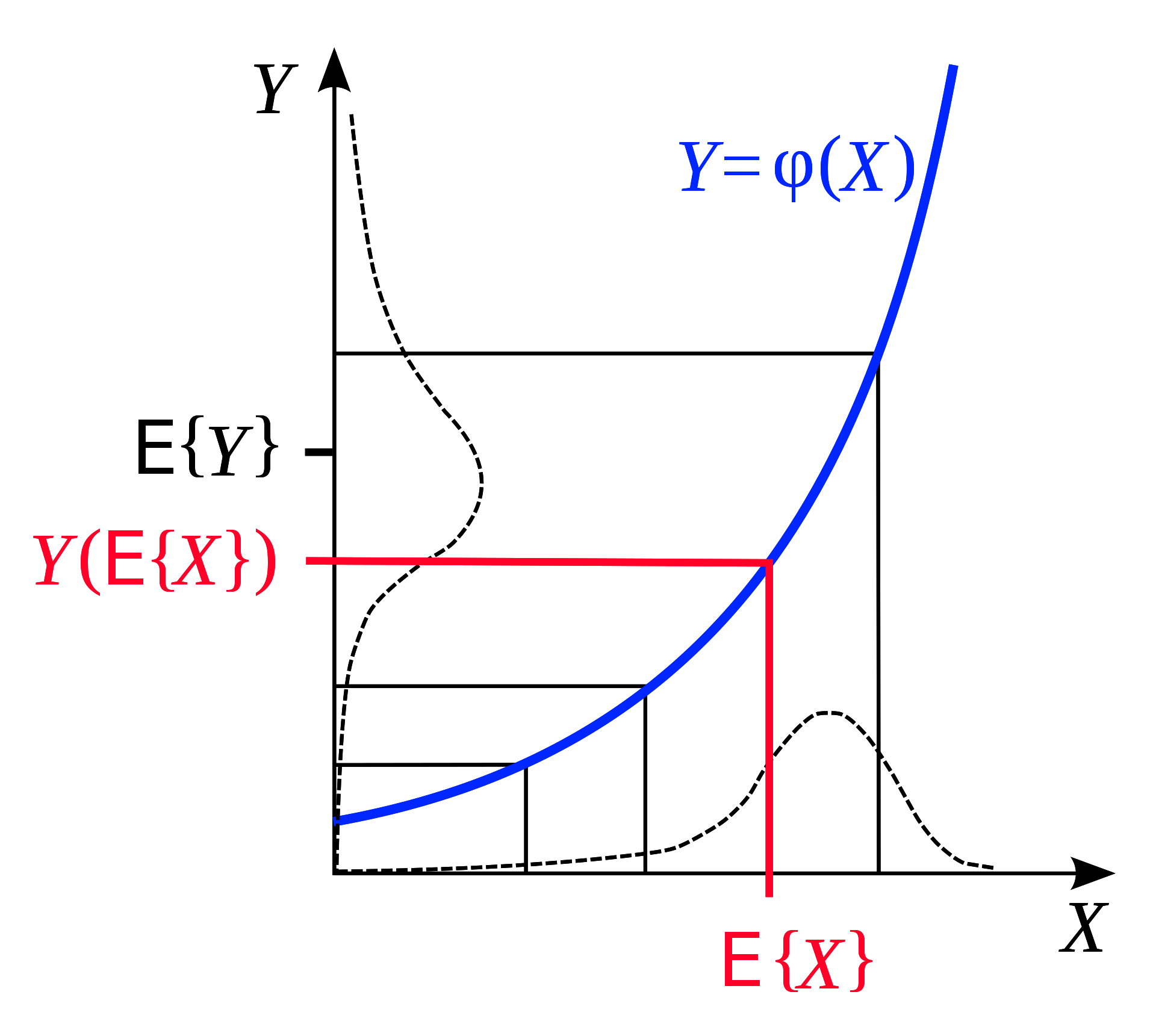
Figure 6: Jensen's Inequality (taken from [Wikipedia](https://en.wikipedia.org/wiki/Jensen%27s_inequality))
Likewise, if $F$ is convex, for a fixed probability distribution $q$, we can infer from Jensen’s Inequality that over the range $z$,
\[F\Bigg(\int_z q(z)h(z)\Bigg) \leq \int_z q(z)F(h(z)) \tag{1}\]Now, recall that our marginalized $L(x,y)$ after multiplication with $\frac{q(z)}{q(z)}$ is,
\[L(x,y) = -\frac{1}{\beta}\int_z q(z) \frac{\exp({-\beta E(x,y,z)})}{q(z)}\]If we make $h(z) = -\frac{1}{\beta} \frac{\exp({-\beta E(x,y,z)})}{q(z)}$, we know from Jensen’s Inequality $(1)$ that
\[F\Bigg(\int_z q(z)\frac{\exp({-\beta E(x,y,z)})}{q(z)}\Bigg) \leq \int_z q(z)F\Bigg(\frac{\exp({-\beta E(x,y,z)})}{q(z)}\Bigg)\]Let’s continue to work this, with a concrete convex loss function, $F(x) = -\log(x)$
\[-\log\Bigg(-\frac{1}{\beta}\int_z q(z)\frac{\exp({-\beta E(x,y,z)})}{q(z)}\Bigg) \leq \int_z q(z) * \frac{-1}{\beta}\log\Bigg(\frac{\exp({-\beta E(x,y,z)})}{q(z)}\Bigg)\] \[\leq \int_z q(z)[E(x,y,z) + \frac{1}{\beta}\log(q(z))]\] \[\leq \int_z q(z)E(x,y,z) + \frac{1}{\beta}\int_z q(z)\log(q(z))\]Great! Now we have an upper bound to our loss function $L(x,y)$, composed of two terms we understand. The first term $\int_z q(z)E(x,y,z)$ is the average energy. And the second term $\frac{1}{\beta}\int_z\log(q(z))$ is just some factor ($-\frac{1}{\beta}$) times the entropy of the distribution $q$.
What’s the point?
We now have formulated an upper bound in such a way that we can avoid complicated integrations, and instead simply approximate these values by sampling from a surrogate distribution ($q(z)$), of our choice!
To get the value of the first term of our upper bound function, we just sample from that distribution, and compute the average value of $L$ that we obtain from applying our sampled $z$’s.
The second term (a factor of entropy) is just a property of the distribution family, and can likewise be approximated with random sampling of $q$.
Finally, we can minimize $L$ with respect to its parameters (say, weights of a network $W$), by minimizing this function that bounds $L$ above. We conduct this minimization by updating our two variables: (1) the entropy of $q$, and (2) our model parameters $W$.
Summary
This is the “energy view” of variational inference. If you need to compute the log of a sum of exponentials, replace it with the average of your function plus an entropy term. This gives us an upper bound. We then minimise this upper bound, and in doing so minimize the function we actually care about.
📝 Yada Pruksachatkun, Ananya Harsh Jha, Joseph Morag, Dan Jefferys-White, and Brian Kelly
4 May 2020