Graph Convolutional Networks III

Introduction to Graph Convolutional Network (GCN)

Graph Convolutional Network (GCN) is one type of architecture that utilizes the structure of data. Before going into details, let’s have a quick recap on self-attention, as GCN and self-attention are conceptually relevant.

Recap: Self-attention

• In self-attention, we have a set of input $\lbrace\boldsymbol{x}_{i}\rbrace^{t}_{i=1}$. Unlike a sequence, it does not have an order.
• Hidden vector $\boldsymbol{h}$ is given by linear combination of the vectors in the set.
• We can express this as $\boldsymbol{X}\boldsymbol{a}$ using matrix vector multiplication, where $\boldsymbol{a}$ contains coefficients that scale the input vector $\boldsymbol{x}_{i}$.

For a detailed explanation, refer to the notes of Week 12.

Notation

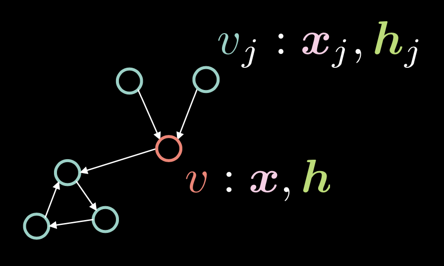
Fig. 1: Graph Convolutional Network

In Figure 1, vertex $v$ is comprised of two vectors: input $\boldsymbol{x}$ and its hidden representation $\boldsymbol{h}$. We also have multiple vertices $v_{j}$, which is comprised of $\boldsymbol{x}_j$ and $\boldsymbol{h}_j$. In this graph, vertices are connected with directed edges.

We represent these directed edges with adjacency vector $\boldsymbol{a}$, where each element $\alpha_{j}$ is set to $1$ if there is a directed edge from $v_{j}$ to $v$.

The degree (number of incoming edges) $d$ is defined as the norm of this adjacency vector, i.e. $\Vert\boldsymbol{a}\Vert_{1} $, which is the number of ones in the vector $\boldsymbol{a}$.

The hidden vector $\boldsymbol{h}$ is given by the following expression:

where $f(\cdot)$ is a non-linear function such as ReLU $(\cdot)^{+}$, Sigmoid $\sigma(\cdot)$, and hyperbolic tangent $\tanh(\cdot)$.

The $\boldsymbol{U}\boldsymbol{x}$ term takes into account the vertex $v$ itself, by applying rotation $\boldsymbol{U}$ to the input $v$.

Remember that in self-attention, the hidden vector $\boldsymbol{h}$ is computed by $\boldsymbol{X}\boldsymbol{a}$, which means that the columns in $\boldsymbol{X}$ is scaled by the factors in $\boldsymbol{a}$. In the context of GCN, this means that if we have multiple incoming edges,i.e. multiple ones in adjacency vector $\boldsymbol{a}$, $\boldsymbol{X}\boldsymbol{a}$ gets larger. On the other hand, if we have only one incoming edge, this value gets smaller. To remedy this issue of the value being proportionate to the number of incoming edges, we divide it by the number of incoming edges $d$. We then apply rotation $\boldsymbol{V}$ to $\boldsymbol{X}\boldsymbol{a}d^{-1}$.

We can represent this hidden representation $\boldsymbol{h}$ for the entire set of inputs $\boldsymbol{x}$ using the following matrix notation:

where $\vect{D} = \text{diag}(d_{i})$.

Residual Gated GCN Theory and Code

Residual Gated Graph Convolutional Network is a type of GCN that can be represented as shown in Figure 2:

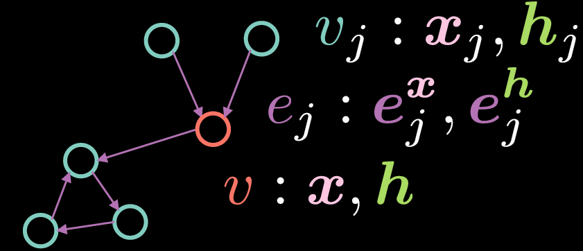
Fig. 2: Residual Gated Graph Convolutional Network

As with the standard GCN, the vertex $v$ consists of two vectors: input $\boldsymbol{x}$ and its hidden representation $\boldsymbol{h}$. However, in this case, the edges also have a feature representation, where $\boldsymbol{e_{j}^{x}}$ represents the input edge representation and $\boldsymbol{e_{j}^{h}}$ represents the hidden edge representation.

The hidden representation $\boldsymbol{h}$ of the vertex $v$ is computed by the following equation:

where $\boldsymbol{x}$ is the input representation, $\boldsymbol{Ax}$ represents a rotation applied to the input $\boldsymbol{x}$ and $\sum_{v_j→v}{\eta(\boldsymbol{e_{j}})\odot \boldsymbol{Bx_{j}}}$ denotes the summation of elementwise multiplication of rotated incoming features $\boldsymbol{Bx_{j}}$ and a gate $\eta(\boldsymbol{e_{j}})$. In contrast to the standard GCN above where we average the incoming representations, the gate term is critical to the implementation of Residual Gated GCN since it allows us to modulate the incoming representations based on the edge representations.

Note that the summation is only over vertices ${v_j}$ that have incoming edges to vertex ${v}$. The term residual (in Residual Gated GCN) comes from the fact that in order to calculate the hidden representation $\boldsymbol{h}$, we add the input representation $\boldsymbol{x}$. The gate term $\eta(\boldsymbol{e_{j}})$ is calculated as shown below:

The gate value $\eta(\boldsymbol{e_{j}})$ is a normalized sigmoid obtained by dividing the sigmoid of the incoming edge representation by the sum of sigmoids of all incoming edge representations. Note that in order to calculate the gate term, we need the representation of the edge $\boldsymbol{e_{j}}$, which can be computed using the equations below:

The hidden edge representation $\boldsymbol{e_{j}^{h}}$ is obtained by the summation of the initial edge representation $\boldsymbol{e_{j}^{x}}$ and $\texttt{ReLU}(\cdot)$ applied to $\boldsymbol{e_{j}}$ where $\boldsymbol{e_{j}}$ is in turn given by the summation of a rotation applied to $\boldsymbol{e_{j}^{x}}$, a rotation applied to the input representation $\boldsymbol{x_{j}}$ of the vertex $v_{j}$ and a rotation applied to the input representation $\boldsymbol{x}$ of the vertex $v$.

Note: In order to calculate hidden representations downstream (e.g.* $2^\text{nd}$ layer hidden representations), we can simply replace the input feature representations by the $1^\text{st}$ layer feature representations in the equations above.*

Graph Classification and Residual Gated GCN Layer

In this section, we introduce the problem of graph classification and code up a Residual Gated GCN layer. In addition to the usual import statements, we add the following:

os.environ['DGLBACKEND'] = 'pytorch'
import dgl
from dgl import DGLGraph
from dgl.data import MiniGCDataset
import networkx as nx

The first line tells DGL to use PyTorch as the backend. Deep Graph Library (DGL) provides various functionalities on graphs whereas networkx allows us to visualise the graphs.

In this notebook, the task is to classify a given graph structure into one of 8 graph types. The dataset obtained from dgl.data.MiniGCDataset yields some number of graphs (num_graphs) with nodes between min_num_v and max_num_v. Hence, all the graphs obtained do not have the same number of nodes/vertices.

Note: In order to familiarize yourself with the basics of DGLGraphs, it is recommended to go through the short tutorial here.

Having created the graphs, the next task is to add some signal to the domain. Features can be applied to nodes and edges of a DGLGraph. The features are represented as a dictionary of names (strings) and tensors (fields). ndata and edata are syntax sugar to access the feature data of all nodes and edges.

The following code snippet shows how the features are generated. Each node is assigned a value equal to the number of incident edges, whereas each edge is assigned the value 1.

def create_artificial_features(dataset):
    for (graph, _) in dataset:
        graph.ndata['feat'] = graph.in_degrees().view(-1, 1).float()
        graph.edata['feat'] = torch.ones(graph.number_of_edges(), 1)
    return dataset

Training and testing datasets are created and features are assigned as shown below:

trainset = MiniGCDataset(350, 10, 20)
testset = MiniGCDataset(100, 10, 20)

trainset = create_artificial_features(trainset)
testset = create_artificial_features(testset)

A sample graph from the trainset has the following representation. Here, we observe that the graph has 15 nodes and 45 edges and both the nodes and edges have a feature representation of shape (1,) as expected. Furthermore, the 0 signifies that this graph belongs to class 0.

(DGLGraph(num_nodes=15, num_edges=45,
         ndata_schemes={'feat': Scheme(shape=(1,), dtype=torch.float32)}
         edata_schemes={'feat': Scheme(shape=(1,), dtype=torch.float32)}), 0)

Note about DGL Message and Reduce Functions

In DGL, the message functions are expressed as Edge UDFs (User Defined Functions). Edge UDFs take in a single argument edges. It has three members src, dst, and data for accessing source node features, destination node features, and edge features respectively. The reduce functions are Node UDFs. Node UDFs have a single argument nodes, which has two members data and mailbox. data contains the node features and mailbox contains all incoming message features, stacked along the second dimension (hence the dim=1 argument). update_all(message_func, reduce_func) sends messages through all edges and updates all nodes.

Gated Residual GCN Layer Implementation

A Gated Residual GCN layer is implemented as shown in the code snippets below.

Firstly, all the rotations of the input features $\boldsymbol{Ax}$, $\boldsymbol{Bx_{j}}$, $\boldsymbol{Ce_{j}^{x}}$, $\boldsymbol{Dx_{j}}$ and $\boldsymbol{Ex}$ are computed by defining nn.Linear layers inside the __init__ function and then forward propagating the input representations h and e through the linear layers inside the forward function.

class GatedGCN_layer(nn.Module):

    def __init__(self, input_dim, output_dim):
        super().__init__()
        self.A = nn.Linear(input_dim, output_dim)
        self.B = nn.Linear(input_dim, output_dim)
        self.C = nn.Linear(input_dim, output_dim)
        self.D = nn.Linear(input_dim, output_dim)
        self.E = nn.Linear(input_dim, output_dim)
        self.bn_node_h = nn.BatchNorm1d(output_dim)
        self.bn_node_e = nn.BatchNorm1d(output_dim)

Secondly, we compute the edge representations. This is done inside the message_func function, which iterates over all the edges and computes the edge representations. Specifically, the line e_ij = edges.data['Ce'] + edges.src['Dh'] + edges.dst['Eh'] computes (Eq. 7) from above. The message_func function ships Bh_j (which is $\boldsymbol{Bx_{j}}$ from (Eq. 5)) and e_ij (Eq. 7) through the edge into the destination node’s mailbox.

def message_func(self, edges):
    Bh_j = edges.src['Bh']
    # e_ij = Ce_ij + Dhi + Ehj
    e_ij = edges.data['Ce'] + edges.src['Dh'] + edges.dst['Eh']
    edges.data['e'] = e_ij
    return {'Bh_j' : Bh_j, 'e_ij' : e_ij}

Thirdly, the reduce_func function collects the shipped messages by the message_func function. After collecting the node data Ah and shipped data Bh_j and e_ij from the mailbox, the line h = Ah_i + torch.sum(sigma_ij * Bh_j, dim=1) / torch.sum(sigma_ij, dim=1) computes the hidden representation of each node as indicated in (Eq. 5). Note however, that this only represents the term $(\boldsymbol{Ax} + \sum_{v_j→v}{\eta(\boldsymbol{e_{j}})\odot \boldsymbol{Bx_{j}}})$ without the $\texttt{ReLU}(\cdot)$ and residual connection.

def reduce_func(self, nodes):
    Ah_i = nodes.data['Ah']
    Bh_j = nodes.mailbox['Bh_j']
    e = nodes.mailbox['e_ij']
    # sigma_ij = sigmoid(e_ij)
    sigma_ij = torch.sigmoid(e)
    # hi = Ahi + sum_j eta_ij * Bhj
    h = Ah_i + torch.sum(sigma_ij * Bh_j, dim=1) / torch.sum(sigma_ij, dim=1)
    return {'h' : h}

Inside the forward function, having called g.update_all, we obtain the results of graph convolution h and e, which represent the terms $(\boldsymbol{Ax} + \sum_{v_j→v}{\eta(\boldsymbol{e_{j}})\odot \boldsymbol{Bx_{j}}})$ from (Eq.5) and $\boldsymbol{e_{j}}$ from (Eq. 7) respectively. Then, we normalize h and e with respect to the graph node size and graph edge size respectively. Batch normalization is then applied so that we can train the network effectively. Finally, we apply $\texttt{ReLU}(\cdot)$ and add the residual connections to obtain the hidden representations for the nodes and edges, which are then returned by the forward function.

def forward(self, g, h, e, snorm_n, snorm_e):

    h_in = h # residual connection
    e_in = e # residual connection

    g.ndata['h']  = h
    g.ndata['Ah'] = self.A(h)
    g.ndata['Bh'] = self.B(h)
    g.ndata['Dh'] = self.D(h)
    g.ndata['Eh'] = self.E(h)
    g.edata['e']  = e
    g.edata['Ce'] = self.C(e)

    g.update_all(self.message_func, self.reduce_func)

    h = g.ndata['h'] # result of graph convolution
    e = g.edata['e'] # result of graph convolution

    h = h * snorm_n # normalize activation w.r.t. graph node size
    e = e * snorm_e # normalize activation w.r.t. graph edge size

    h = self.bn_node_h(h) # batch normalization
    e = self.bn_node_e(e) # batch normalization

    h = torch.relu(h) # non-linear activation
    e = torch.relu(e) # non-linear activation

    h = h_in + h # residual connection
    e = e_in + e # residual connection

    return h, e

Next, we define the MLP_Layer module which contains several fully connected layers (FCN). We create a list of fully connected layers and forward through the network.

Finally, we define our GatedGCN model which comprises of the previously defined classes: GatedGCN_layer and MLP_layer. The definition of our model (GatedGCN) is shown below.

 class GatedGCN(nn.Module):
    def __init__(self, input_dim, hidden_dim, output_dim, L):
        super().__init__()
        self.embedding_h = nn.Linear(input_dim, hidden_dim)
        self.embedding_e = nn.Linear(1, hidden_dim)
        self.GatedGCN_layers = nn.ModuleList([
            GatedGCN_layer(hidden_dim, hidden_dim) for _ in range(L)
        ])
        self.MLP_layer = MLP_layer(hidden_dim, output_dim)
    def forward(self, g, h, e, snorm_n, snorm_e):
        # input embedding
        h = self.embedding_h(h)
        e = self.embedding_e(e)
        # graph convnet layers
        for GGCN_layer in self.GatedGCN_layers:
            h, e = GGCN_layer(g, h, e, snorm_n, snorm_e)
        # MLP classifier
        g.ndata['h'] = h
        y = dgl.mean_nodes(g,'h')
        y = self.MLP_layer(y)
        return y

In our constructor, we define the embeddings for e and h (self.embedding_e and self.embedding_h), self.GatedGCN_layers which is list (of size $L$) of our previously defined model: GatedGCN_layer, and finally self.MLP_layer which was also defined before. Next, using these initializations, we simply forward through the model and output y.

To better understand the model, we initiate an object of the model and print it for better visualization:

# instantiate network
model = GatedGCN(input_dim=1, hidden_dim=100, output_dim=8, L=2)
print(model)

The main structure of the model is shown below:

GatedGCN(
  (embedding_h): Linear(in_features=1, out_features=100, bias=True)
  (embedding_e): Linear(in_features=1, out_features=100, bias=True)
  (GatedGCN_layers): ModuleList(
    (0): GatedGCN_layer(...)
    (1): GatedGCN_layer(... ))
  (MLP_layer): MLP_layer(
    (FC_layers): ModuleList(...))

Not surprisingly, we have two layers of GatedGCN_layer (since L=2) followed by a MLP_layer which finally yields an output of 8 values.

Moving on, we define our train and evaluate functions. In our train function, we have our generic code which takes samples from dataloader. Next, batch_graphs, batch_x, batch_e, batch_snorm_n and batch_snorm_e are fed into our model which returns batch_scores (of size 8). The predicted scores are compared with the ground truth in our loss function: loss(batch_scores, batch_labels). Then, we zero out gradients (optimizer.zero_grad()), perform backprop (J.backward()) and updates our weights (optimizer.step()). Finally, loss for epoch and training accuracy is calculated. Furthermore, we use a similar code for our evaluate function.

Finally, we are ready to train! We found that after 40 epochs of training, our model has learned to classify the graphs with a test accuracy of $87$%.