Energy-Based Models

Overview

We will introduce a new framework for defining models. It provides a unifying umbrella that helps define supervised, unsupervised and self-supervised models. Energy-based models observe a set of variables $x$ and output a set of variables $y$. There are 2 major problems with feed-forward nets:

1. What if the inference procedure is a more complex calculation than stacked layers of weighted sums?
2. What if there are multiple possible outputs for a single input? Example: Predicting future frames of video. Essentially in a classification net, we train this net to emit a score for each class. However, this is not possible to do in a continuous high dimensional domain like images. (We cannot have softmax over images!). Even if the output is discrete, it could have a large sample space. For example, the text is compositional leading to a huge number of possible combinations. Energy-based models provide a better framework to model these modalities.

EBM approach

Instead of trying to classify $x$’s to $y$’s, we would like to predict if a certain pair of ($x$, $y$) fit together or not. Or in other words, find a $y$ compatible with $x$. We can also pose the problem as finding a $y$ for which some $F(x,y)$ is low. For example:

• Is $y$ an accurate high-resolution image of $x$ ?
• Is text A a good translation of text B?

Definition

We define an energy function $F: \mathcal{X} \times \mathcal{Y} \rightarrow \mathcal{R}$ where $F(x,y)$ describes the level of dependency between $(x,y)$ pairs. (Note that this energy is used in inference, not in learning.) The inference is given by the following equation:

Solution: gradient-based inference

We would like the energy function to be smooth and differentiable so that we can use it to perform the gradient-based method for inference. In order to perform inference, we search this function using gradient descent to find compatible $y$’s. There are many alternate methods to gradient methods to obtain the minimum.

Aside: Graphical models are a special case of Energy-Based models. The energy function decomposes as a sum of energy terms. Each energy terms take into account a subset of variables that we are dealing with. If they organize in a particular form, there are efficient inference algorithms to find the minimum of the sum of the terms with respect to the variable that we are interested in inferring.

EBM with latent variables

The output $y$ depends on $x$ as well as an extra variable $z$ (the latent variable) which we do not know the value of. These latent variables can provide auxiliary information. For example, a latent variable can tell you the positions of word boundaries in a chunk of text. This would be helpful to know when we want to interpret handwriting without spaces. This is also especially useful to know in speech that can have hard-to-decipher gaps. Additionally, some languages have very faint word boundaries (e.g. French). Hence, having this latent variable in our model will be very useful to interpret such an input.

Inference

To do inference with latent variable EBM, we want to simultaneously minimize energy function with respect to y and z.

And this is equivalent to redefining the energy function as: \(F_\infty(x,y) = \text{argmin}_{z}E(x,y,z)\), which equals to: \(F_\beta(x,y) = -\frac{1}{\beta}\log\int_z \exp(-\beta E(x,y,z))\). When $\beta \rightarrow \infty$, then $\check{y} = \text{argmin}_{y}F(x,y)$.

Another big advantage of allowing latent variables, is that by varying the latent variable over a set, we can make the prediction output $y$ vary over the manifold of possible predictions as well (the ribbon is shown in the graph below): $F(x,y) = \text{argmin}_{z} E(x,y,z)$.

This allows a machine to produce multiple outputs, not just one.

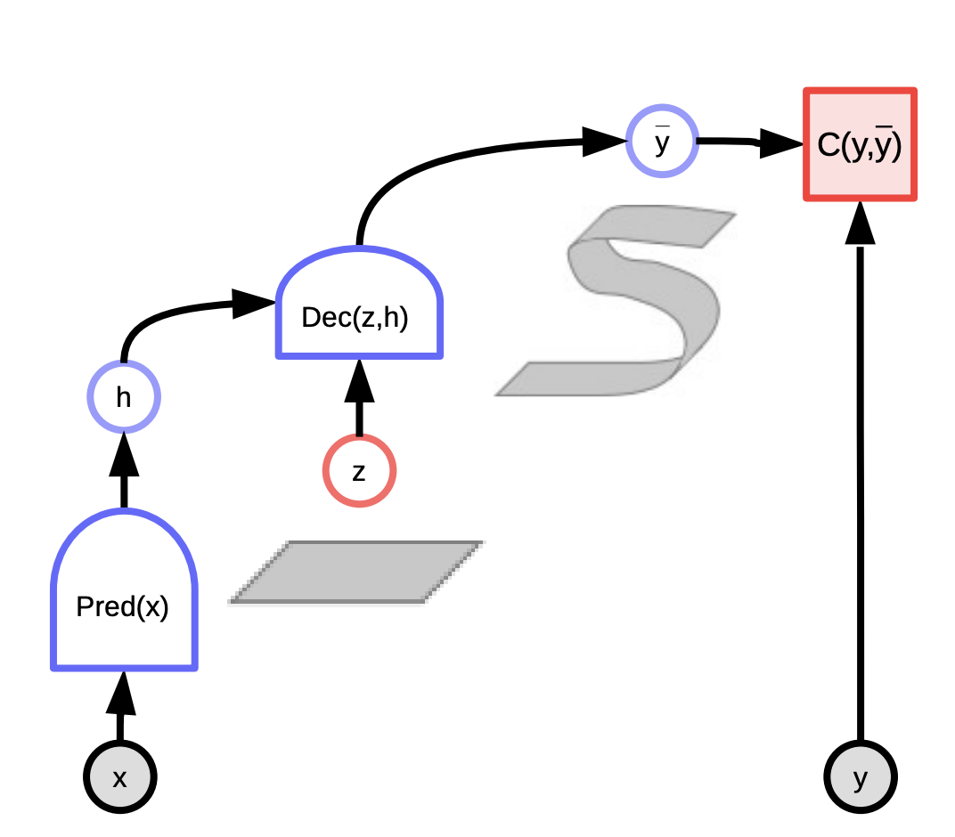
Fig. 1: Computation graph for Energy-based models

Examples

One example is video prediction. There are many good applications for us to use video prediction, one example is to make a video compression system. Another is to use video taken from a self-driving car and predict what other cars are going to do.

Another example is translation. Language translation has always been a difficult problem because there is no single correct translation for a piece of text from one language to another. Usually, there are a lot of different ways to express the same idea and people find it is hard to reason why they pick one over the other. So it might be nice if we have some way of parametrising all the possible translations that a system could produce to respond to a given text. Let’s say if we want to translate German to English, there could be multiple translations in English that are all correct, and by varying some latent variables then you may vary the translation produced.

Energy-based models v.s. probabilistic models

We can look at the energies as unnormalised negative log probabilities, and use Gibbs-Boltzmann distribution to convert from energy to probability after normalization is:

where $\beta$ is positive constant and needs to be calibrated to fit your model: as $\beta \rightarrow \infty$, this function converges to the argmax function; smaller values of $\beta$ leads to a smoother distribution. (In physics, $\beta$ is inverse temperature: $\beta \rightarrow \infty$ means temperature goes to zero).

Now if marginalize over y: $P(y \mid x) = \int_z P(y,z \mid x)$, we have:

Thus, if we have a latent variable model and want to eliminate the latent variable $z$ in a probabilistically correct way, we just need to redefine the energy function $F_\beta$ (Free Energy)

Free Energy

Computing this can be very hard… In fact, in most cases, it’s probably intractable. So if you have a latent variable that you want to minimize over inside of your model, or if you have a latent variable that you want to marginalize over (which you do by defining this Energy function $F$), and minimizing corresponds to the infinite $\beta$ limit of this formula, then it can be done.

Under the definition of $F_\beta(x, y)$ above, $P(y \mid x)$ is just an application of the Gibbs-Boltzmann formula and $z$ has been marginalized implicitly inside of this. Physicists call this “Free Energy”, which is why we call it $F$. So $e$ is the energy, and $F$ is free energy.

Question: Can you elaborate on the advantage that energy-based models give? In probability-based models, you can also have latent variables, which can be marginalized over.

The difference is that in probabilistic models, you basically don’t have the choice of the objective function you’re going to minimize, and you have to stay true to the probabilistic framework in the sense that every object you manipulate has to be a normalized distribution (which you may approximate using variational methods, etc.). Here, we’re saying that ultimately what you want to do with these models is make decisions. If you build a system that drives a car, and the system tells you “I need to turn left with probability 0.8 or turn right with probability 0.2”, you’re going to turn left. The fact that the probabilities are 0.2 and 0.8 doesn’t matter – what you want is to make the best decision, because you’re forced to make a decision. So probabilities are useless if you want to make decisions. If you want to combine the output of an automated system with another one (for example, a human, or some other system), and these systems haven’t been trained together, but rather they have been trained separately, then what you want are calibrated scores so that you can combine the scores of the two systems so that you can make a good decision. There is only one way to calibrate scores, and that is to turn them into probabilities. All other ways are either inferior or equivalent. But if you’re going to train a system end-to-end to make decisions, then whatever scoring function you use is fine, as long as it gives the best score to the best decision. Energy-based models give you way more choices in how you handle the model, way more choices of how you train it, and what objective function you use. If you insist your model be probabilistic, you have to use maximum likelihood – you basically have to train your model in such a way that the probability it gives to the data you observed is maximum. The problem is that this can only be proven to work in the case where your model is “correct” – and your model is never “correct”. There’s a quote from a famous statistician [Goerge Box] that says “All models are wrong, but some are useful.” So probabilistic models, particularly those in high-dimensional spaces, and in combinatorial spaces such as text, are all approximate models. They’re all wrong in a way, and if you try to normalize them, you make them more wrong. So you’re better off not normalizing them.

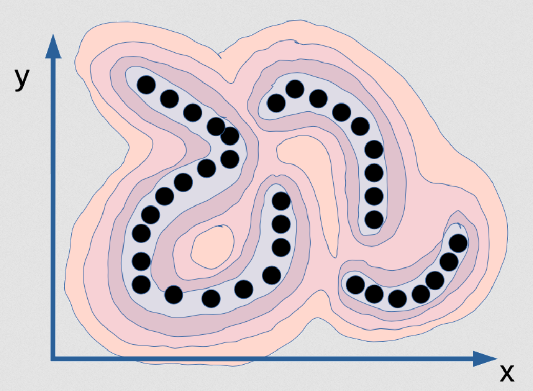
Fig. 2: Visualization of the energy function that captures dependency between x and y

This is an energy function that’s meant to capture the dependency between x and y. It’s like a mountain range if you will. The valleys are where the black dots are (these are data points), and there are mountains all around. Now, if you train a probabilistic model with this, imagine that the points are actually on an infinitely thin manifold. So the data distribution for the black dots is actually just a line, and there are three of them. They don’t actually have any width. So if you train a probabilistic model on this, your density model should tell you when you are on this manifold. On this manifold, the density is infinite, and just $\varepsilon$ outside of it should be zero. That would be the correct model of this distribution. Not only should the density be infinite, but the integral over [x and y] should be 1. This is very difficult to implement on the computer! Not only that, but it’s also basically impossible. Let’s say you want to compute this function through some sort of neural net – your neural net will have to have infinite weights, and they would need to be calibrated in such a way that the integral of the output of that system over the entire domain is 1. That’s basically impossible. The accurate, correct probabilistic model for this particular data example is impossible. This is what maximum likelihood will want you to produce, and there’s no computer in the world that can compute this. So in fact, it’s not even interesting. Imagine that you had the perfect density model for this example, which is a thin plate in that (x, y) space – you couldn’t do inference! If I give you a value of x, and ask you “what’s the best value of y?” You wouldn’t be able to find it because all values of y except a set of zero-probability have a probability of zero, and there are just a few values that are possible. For these values of x for example:

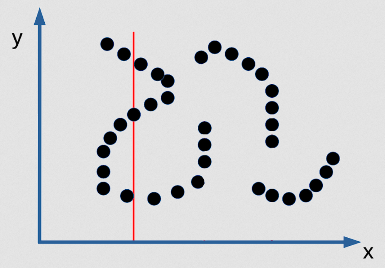
Fig. 3: Example for multiple prediction of EBM as an implicit function

There are 3 values of y that are possible, and they are infinitely narrow. So you wouldn’t be able to find them. There’s no inference algorithm that will allow you to find them. The only way you can find them is if you make your contrast function smooth and differentiable, and then you can start from any point and by gradient descent you can find a good value for y for any value of x. But this is not going to be a good probabilistic model of the distribution if the distribution is of the type I mentioned. So here is a case where insisting to have a good probabilistic model is actually bad. Maximum likelihood sucks [in this case]!

So if you are a true Bayesian, you say “oh but you can correct this by having a strong prior where the prior says your density function has to be smooth”. You could think of this as a prior. But, everything you do in Bayesian terms – take the logarithm thereof, forget about normalization – you get energy-based models. Energy-based models that have a regulariser, which is additive to your energy function, are completely equivalent to Bayesian models where the likelihood is exponential of the energy, and now you get $\exp(\text{energy}) \exp(\text{regulariser})$, and so it’s equal to $\exp(\text{energy} + \text{regulariser})$. And if you remove the exponential you have an energy-based model with an additive regulariser.

So there is a correspondence between probabilistic and Bayesian methods there, but insisting that you do maximum likelihood is sometimes bad for you, particularly in high-dimensional spaces or combinatorial spaces where your probabilistic model is very wrong. It’s not very wrong in discrete distributions (it’s okay) but in continuous cases, it can be really wrong. And all the models are wrong.