SSL, EBM with details and examples

Self supervised learning

Self Supervised Learning (SSL) encompasses both supervised and unsupervised learning. The objective of the SSL pretext task is to learn a good representation of the input so that it can subsequently be used for supervised tasks. In SSL, the model is trained to predict one part of the data given other parts of the data. For example, BERT was trained using SSL techniques and the Denoising Auto-Encoder (DAE) has particularly shown state-of-the-art results in Natural Language Processing (NLP).

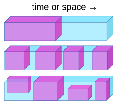
Fig. 1: Self Supervised Learning

Self Supervised Learning task can be defined as the following:

• Predict the future from the past.
• Predict the masked from the visible.
• Predict any occluded parts from all available parts.

For example, if a system is trained to predict the next frame when the camera is moved, the system will implicitly learn about the depth and parallax. This will force the system to learn that objects occluded from its vision do not disappear but continue to exist and the distinction between animate, inanimate objects, and the background. It can also end up learning about intuitive physics like gravity.

State-of-the-art NLP systems (BERT) pre-train a giant neural network on an SSL task. You remove some of the words from a sentence and make the system predict the missing words. This has been very successful. Similar ideas were also tried out in computer vision realm. As shown in the image below, you can take an image and remove a portion of the image and train the model to predict the missing portion.

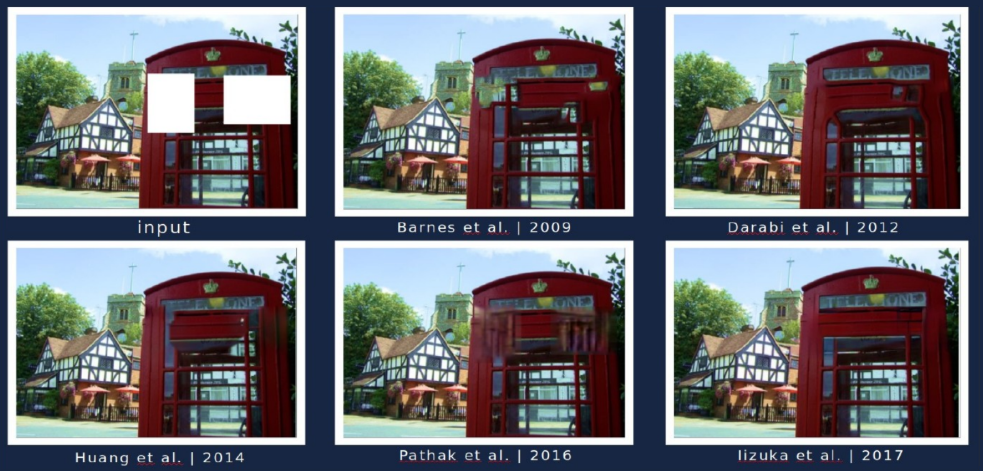
Fig. 2: Corresponding results in computer vision

Although the models can fill in the missing space they have not shared the same level of success as NLP systems. If you were to take the internal representations generated by these models, as input to a computer vision system, it is unable to beat a model that was pre-trained in a supervised manner on ImageNet. The difference here is that NLP is discrete whereas images are continuous. The difference in success is because in the discrete domain we know how to represent uncertainty, we can use a big softmax over the possible outputs, in the continuous domain we do not.

An intelligent system (AI agent) needs to be able to predict the results of its own action on the surroundings and itself to make intelligent decisions. Since the world is not completely deterministic and there is not enough compute power in a machine/human brain to account for every possibility, we need to teach AI systems to predict in the presence of uncertainty in high dimensional spaces. Energy-based models (EBMs) can be extremely useful for this.

A neural network trained using Least Squares to predict the next frame of a video will result in blurry images because the model cannot exactly predict the future so it learns to average out all possibilities of the next frame from the training data to reduce the loss.

Latent variable energy-based models as a solution to make predictions for next frame:

Unlike linear regression, Latent variable energy-based models take what we know about the world as well as a latent variable which gives us information about what happened in reality. A combination of those two pieces of information can be used to make a prediction that will be close to what actually occurs.

These models can be thought of as systems that rate compatibility between the input $x$ and actual output $y$ depending on the prediction using the latent variable that minimizes the energy of the system. You observe input $x$ and produce possible predictions $\bar{y}$ for different combinations of input $x$ and latent variables $z$ and choose the one that minimizes the energy, prediction error, of the system.

Depending upon the latent variable we draw, we can end up with all the possible predictions. The latent variable could be thought of as a piece of important information about the output $y$ that is not present in the input $x$.

Scalar-valued energy function can take two versions:

1. Conditional $F(x, y)$ - measure the compatibility between $x$ and $y$
2. Unconditional $F(y)$ - measure the compatibility between the components of $y$

Training an Energy-Based Model

There are two classes of learning models to train an Energy-Based Model to parametrize $F(x, y)$.

1. Contrastive methods: Push down on $F(x[i], y[i])$, push up on other points $F(x[i], y’)$
2. Architectural Methods: Build $F(x, y)$ so that the volume of low energy regions is limited or minimized through regularization

There are seven strategies to shape the energy function. The contrastive methods differ in the way they pick the points to push up. While the architectural methods differ in the way they limit the information capacity of the code.

An example of the contrastive method is Maximum Likelihood learning. The energy can be interpreted as an unnormalised negative log density. Gibbs distribution gives us the likelihood of $y$ given $x$. It can be formulated as follows:

Maximum likelihood tries to make the numerator big and the denominator small to maximize the likelihood. This is equivalent to minimizing $-\log(P(Y \mid W))$ which is given below

Gradient of the negative log likelihood loss for one sample Y is as follows:

In the above gradient, the first term of the gradient at the data point $Y$ and the second term of the gradient gives us the expected value of the gradient of the energy over all $Y$s. Hence, when we perform gradient descent the first term tries to reduce energy given to the data point $Y$ and the second term tries to increase the energy given to all other $Y$s.

The gradient of the energy function is generally very complex and hence computing, estimating or approximating the integral is a very interesting case as it is intractable in most of the cases.

Latent variable energy-based model

The main advantage of Latent variable models is that they allow multiple predictions through the latent variable. As $z$ varies over a set, $y$ varies over the manifold of possible predictions. Some examples include:

1. K-means
2. Sparse modelling
3. GLO

These can be of two types:

1. Conditional models where $y$ depends on $x$
   1. \[F(x,y) = \text{min}_{z} E(x,y,z)\]
   2. \[F_\beta(x,y) = -\frac{1}{\beta}\log\int_z e^{-\beta E(x,y,z)}\]
2. Unconditional models that have scalar-valued energy function, $F(y)$ that measures the compatibility between the components of $y$
   1. \[F(y) = \text{min}_{z} E(y,z)\]
   2. \[F_\beta(y) = -\frac{1}{\beta}\log\int_z e^{-\beta E(y,z)}\]

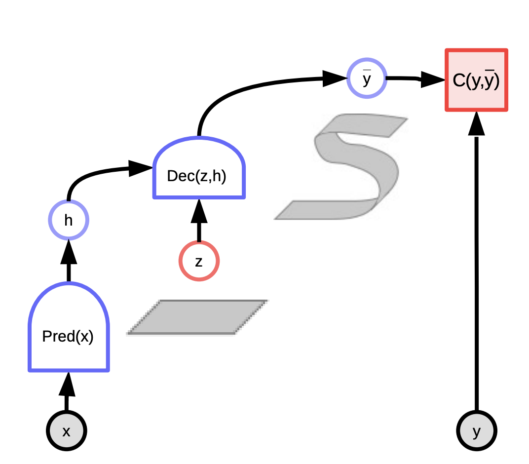
Fig. 3: Latent Variable EBM

Latent variable EBM example: $K$-means

K-means is a simple clustering algorithm that can also be considered as an energy-based model where we are trying to model the distribution over $y$. The energy function is $E(y,z) = \Vert y-Wz \Vert^2$ where $z$ is a $1$-hot vector.

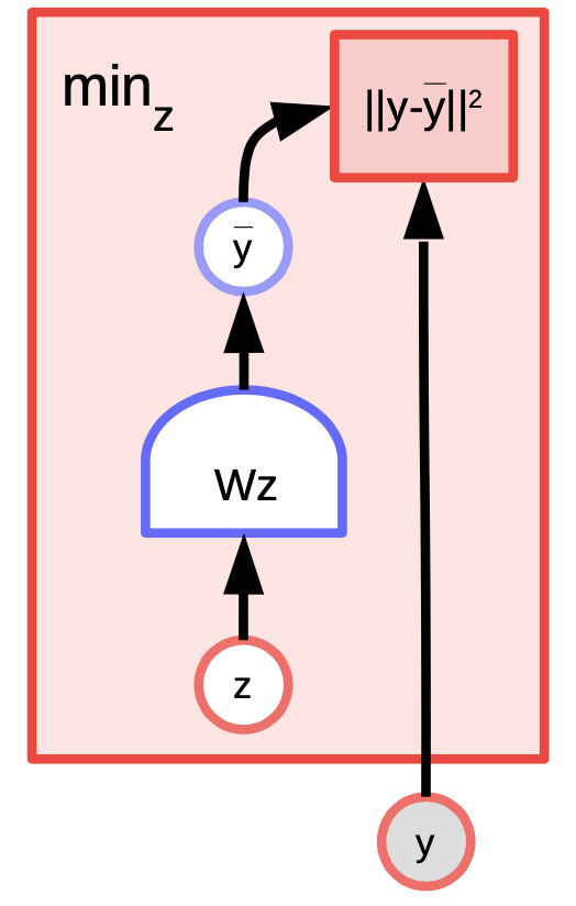
Fig. 4: K-means example

Given a value of $y$ and $k$, we can do inference by figuring out which of the $k$ possible columns of $W$ minimizes the reconstruction error or energy function. To train the algorithm, we can adopt an approach where we can find $z$ to choose the column of $W$ closest to $y$ and then try to get even closer by taking a gradient step and repeat the process. However, coordinate gradient descent actually works better and faster.

In the plot below we can see the data points along the pink spiral. The black blobs surrounding this line corresponds to quadratic wells around each of the prototypes of $W$.

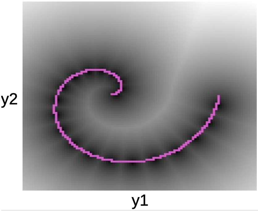
Fig. 5: Spiral plot

Once we learn the energy function, we can begin to address questions like:

1. Given a point $y_1$, can we predict $y_2$?
2. Given $y$, can we find the closest point on the data manifold?

K-means belongs to architectural methods (as opposed to contrastive methods). Hence we do not push up the energy anywhere, all we do is push the energy down in certain regions. One disadvantage is that once the value of $k$ has been decided, there can only be $k$ points that have $0$ energy, and every other point will have higher energy that grows quadratically as we move away from them.

Contrastive methods

According to Dr Yann LeCun, everyone will be using architectural methods at some point, but at this moment, it is contrastive methods that work for images. Consider the figure below which shows us some data points and contours of the energy surface. Ideally, we want the energy surface to have the lowest energy on the data manifold. Hence what we would like to do is lower the energy (i.e. the value of $F(x,y)$) around the training example, but this alone may not be enough. Hence we also raise it for the $y$’s in the region that should have high energy but has low energy.

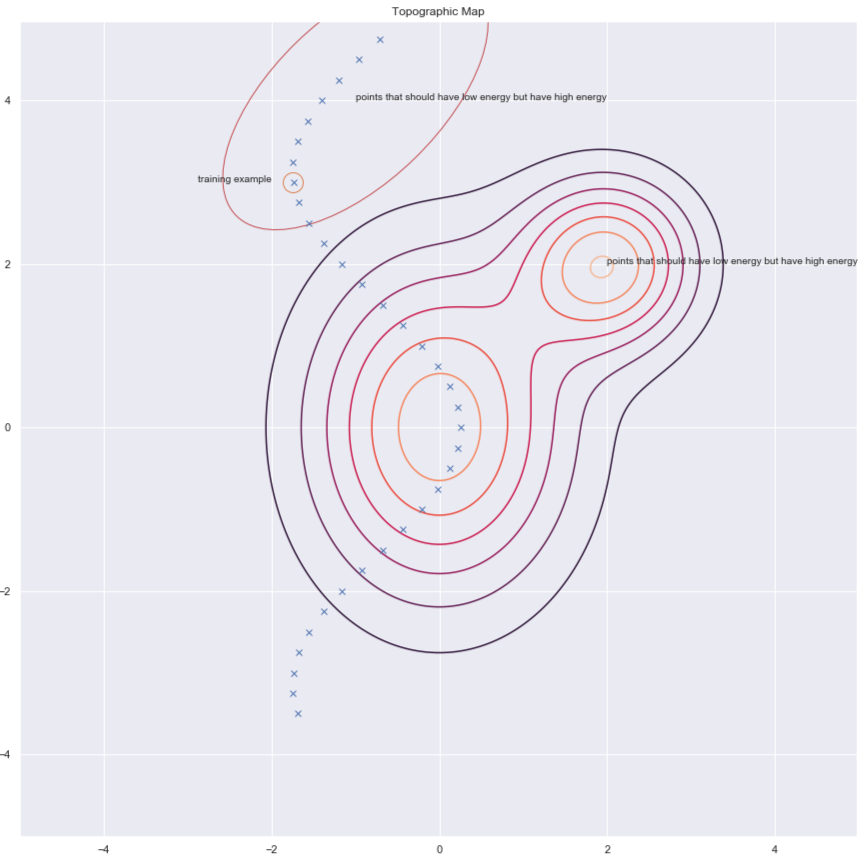
Fig. 6: Contrastive methods

There are several ways to find these candidates $y$’s that we want to raise energy for. Some examples are:

1. Denoising Autoencoder
2. Contrastive Divergence
3. Monte Carlo
4. Markov Chain Monte Carlo
5. Hamiltonian Monte Carlo

We will briefly discuss denoising autoencoders and contrastive divergence.

Denoising autoencoder (DAE)

One way of finding $y$’s to increase energy for it is by randomly perturbing the training example as shown by the green arrows in the plot below.

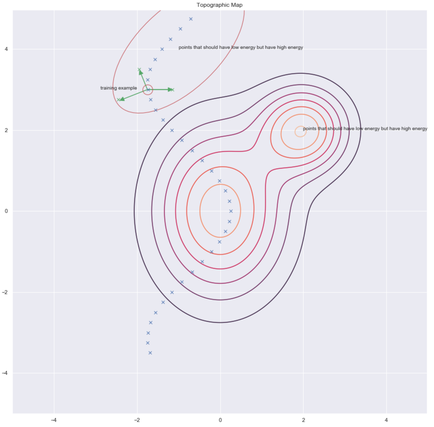
Fig. 7: Topographic map

Once we have a corrupted data point, we can push the energy up here. If we do this sufficiently many times for all the data points, the energy sample will curl up around the training examples. The following plot illustrates how training is done.

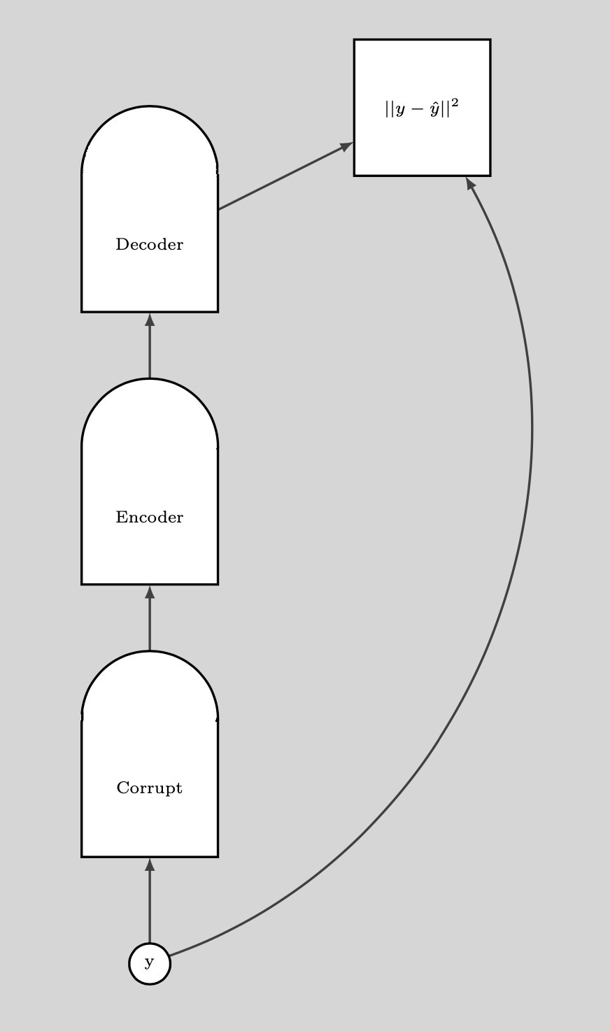
Fig. 8: Training

Steps for training:

1. Take a point $y$ and corrupt it
2. Train the Encoder and Decoder to reconstruct the original data point from this corrupted data point

If the DAE is properly trained, the energy grows quadratically as we move away from the data manifold.

The following plot illustrates how we use the DAE.

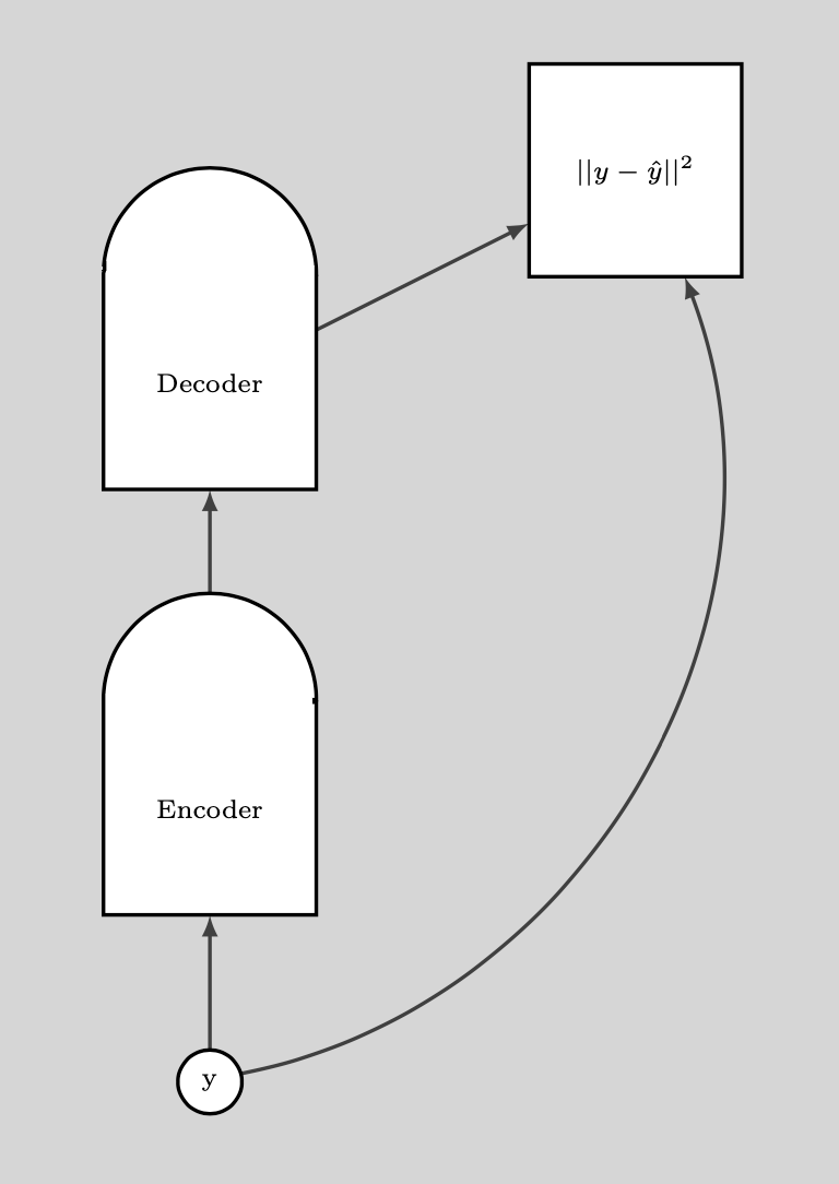
Fig. 9: How DAE is used

BERT

BERT is trained similarly, except that the space is discrete as we are dealing with text. The corruption technique consists of masking some of the words and the reconstruction step consists of trying to predict these. Hence, this is also called a masked autoencoder.

Contrastive divergence

Contrastive Divergence presents us with a smarter way to find the $y$ point that we want to push up the energy for. We can give a random kick to our training point and then move down the energy function using gradient descent. At the end of the trajectory, we push up the energy for the point we land on. This is illustrated in the plot below using the green line.

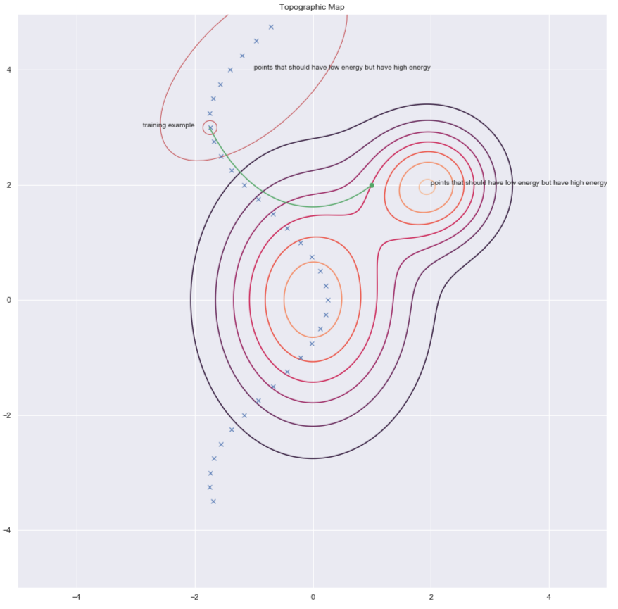
Fig. 10: Contrastive Divergence