Optimisation Techniques I

Gradient descent

We start our study of Optimization Methods with the most basic and the worst (reasoning to follow) method of the lot, Gradient Descent.

Problem:

Iterative Solution:

where,

• $w_{k+1}$ is the updated value after the $k$-th iteration,
• $w_k$ is the initial value before the $k$-th iteration,
• $\gamma_k$ is the step size,
• $\nabla f(w_k)$ is the gradient of $f$.

The assumption here is that the function $f$ is continuous and differentiable. Our aim is to find the lowest point (valley) of the optimization function. However, the actual direction to this valley is not known. We can only look locally, and therefore the direction of the negative gradient is the best information that we have. Taking a small step in that direction can only take us closer to the minimum. Once we have taken the small step, we again compute the new gradient and again move a small amount in that direction, till we reach the valley. Therefore, essentially all that the gradient descent is doing is following the direction of steepest descent (negative gradient).

The $\gamma$ parameter in the iterative update equation is called the step size. Generally we don’t know the value of the optimal step-size; so we have to try different values. Standard practice is to try a bunch of values on a log-scale and then use the best one. There are a few different scenarios that can occur. The image above depicts these scenarios for a 1D quadratic. If the learning rate is too low, then we would make steady progress towards the minimum. However, this might take more time than what is ideal. It is generally very difficult (or impossible) to get a step-size that would directly take us to the minimum. What we would ideally want is to have a step-size a little larger than the optimal. In practice, this gives the quickest convergence. However, if we use too large a learning rate, then the iterates get further and further away from the minima and we get divergence. In practice, we would want to use a learning rate that is just a little less than diverging.

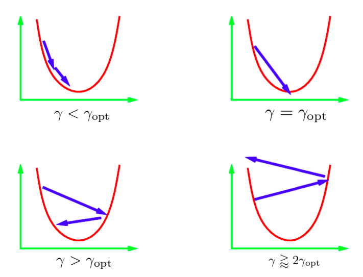
Figure 1: Step sizes for 1D Quadratic

Stochastic gradient descent

In Stochastic Gradient Descent, we replace the actual gradient vector with a stochastic estimation of the gradient vector. Specifically for a neural network, the stochastic estimation means the gradient of the loss for a single data point (single instance).

Let $f_i$ denote the loss of the network for the $i$-th instance.

The function that we eventually want to minimize is $f$, the total loss over all instances.

In SGD, we update the weights according to the gradient over $f_i$ (as opposed to the gradient over the total loss $f$).

If $i$ is chosen randomly, then $f_i$ is a noisy but unbiased estimator of $f$, which is mathematically written as:

As a result of this, the expected $k$-th step of SGD is the same as the $k$-th step of full gradient descent:

Thus, any SGD update is the same as full-batch update in expectation. However, SGD is not just faster gradient descent with noise. Along with being faster, SGD can also get us better results than full-batch gradient descent. The noise in SGD can help us avoid the shallow local minima and find a better (deeper) minima. This phenomenon is called annealing.

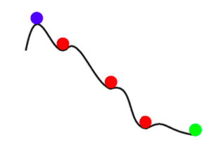
Figure 2: Annealing with SGD

In summary, the advantages of Stochastic Gradient Descent are as follows:

1. There is a lot of redundant information across instances. SGD prevents a lot of these redundant computations.
2. At early stages, the noise is small as compared to the information in the gradient. Therefore a SGD step is virtually as good as a GD step.
3. Annealing - The noise in SGD update can prevent convergence to a bad(shallow) local minima.
4. Stochastic Gradient Descent is drastically cheaper to compute (as you don’t go over all data points).

Mini-batching

In mini-batching, we consider the loss over multiple randomly selected instances instead of calculating it over just one instance. This reduces the noise in the step update.

Often we are able to make better use of our hardware by using mini batches instead of a single instance. For example, GPUs are poorly utilized when we use single instance training. Distributed network training techniques split a large mini-batch between the machines of a cluster and then aggregate the resulting gradients. Facebook recently trained a network on ImageNet data within an hour, using distributed training.

It is important to note that Gradient Descent should never be used with full sized batches. In case you want to train on the full batch-size, use an optimization technique called LBFGS. PyTorch and SciPy both provide implementations of this technique.

Momentum

In Momentum, we have two iterates ($p$ and $w$) instead of just one. The updates are as follows:

$p$ is called the SGD momentum. At each update step we add the stochastic gradient to the old value of the momentum, after dampening it by a factor $\beta$ (value between 0 and 1). $p$ can be thought of as a running average of the gradients. Finally we move $w$ in the direction of the new momentum $p$.

Alternate Form: Stochastic Heavy Ball Method

This form is mathematically equivalent to the previous form. Here, the next step is a combination of previous step’s direction ($w_k - w_{k-1}$) and the new negative gradient.

Intuition

SGD Momentum is similar to the concept of momentum in physics. The optimization process resembles a heavy ball rolling down the hill. Momentum keeps the ball moving in the same direction that it is already moving in. Gradient can be thought of as a force pushing the ball in some other direction.

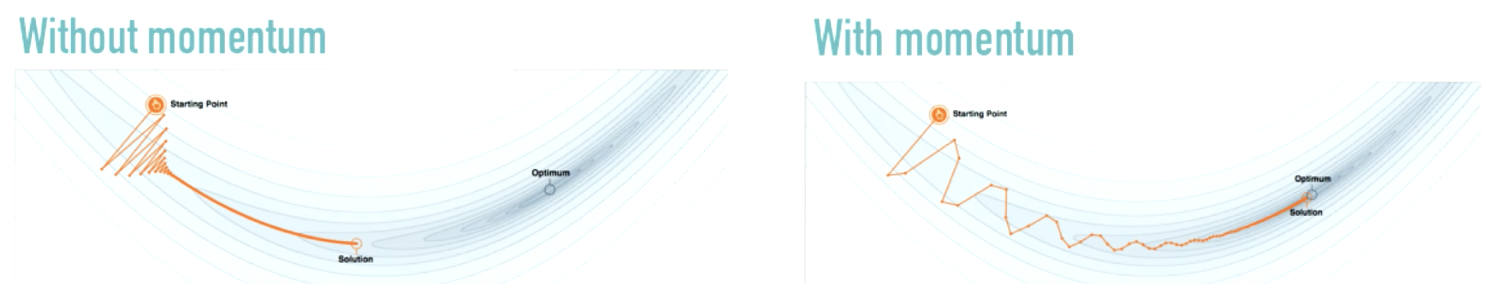
Figure 3: Effect of Momentum
Source: distill.pub

Rather than making dramatic changes in the direction of travel (as in the figure on the left), momentum makes modest changes. Momentum dampens the oscillations which are common when we use only SGD.

The $\beta$ parameter is called the Dampening Factor. $\beta$ has to be greater than zero, because if it is equal to zero, you are just doing gradient descent. It also has to be less than 1, otherwise everything will blow up. Smaller values of $\beta$ result in change in direction quicker. For larger values, it takes longer to make turns.

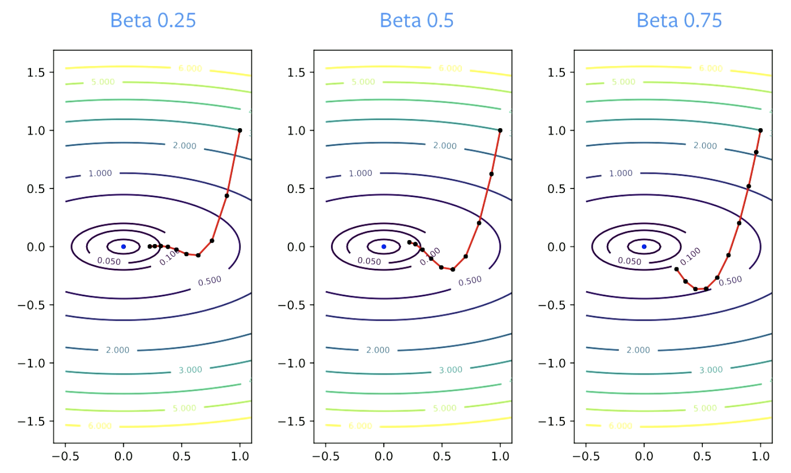
Figure 4: Effect of Beta on Convergence

Practical guidelines

Momentum must pretty much be always be used with stochastic gradient descent. $\beta$ = 0.9 or 0.99 almost always works well.

The step size parameter usually needs to be decreased when the momentum parameter is increased to maintain convergence. If $\beta$ changes from 0.9 to 0.99, learning rate must be decreased by a factor of 10.

Why does momentum works?

Acceleration

The following are the update rules for Nesterov’s momentum.

With Nesterov’s Momentum, you can get accelerated convergence if you choose the constants very carefully. But this applies only to convex problems and not to Neural Networks.

Many people say that normal momentum is also an accelerated method. But in reality, it is accelerated only for quadratics. Also, acceleration does not work well with SGD, as SGD has noise and acceleration does not work well with noise. Therefore, though some bit of acceleration is present with Momentum SGD, it alone is not a good explanation for the high performance of the technique.

Noise smoothing

Probably a more practical and probable reason to why momentum works is Noise Smoothing.

Momentum averages gradients. It is a running average of gradients that we use for each step update.

Theoretically, for SGD to work we should take average over all step updates.

The great thing about SGD with momentum is that this averaging is no longer necessary. Momentum adds smoothing to the optimization process, which makes each update a good approximation to the solution. With SGD you would want to average a whole bunch of updates and then take a step in that direction.

Both Acceleration and Noise smoothing contribute to high performance of momentum.

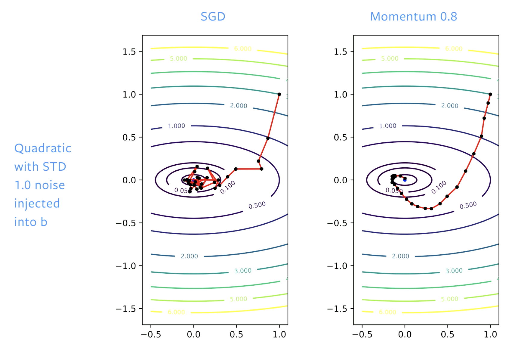
Figure 5: SGD vs. Momentum

With SGD, we make good progress towards solution initially but when we reach bowl (bottom of the valley) we bounce around in this floor. If we adjust learning rate we will bounce around slower. With momentum we smooth out the steps, so that there is no bouncing around.