Training latent variable Energy-Based Models (EBMs)

🎙️ Alfredo Canziani

Free energy

Free energy:

\[F_\infty (\vect{y})=\min_z E(\vect{y},z) = E(\vect{y},\check z)\]

Here, $F_\infty$ is the zero temperature limit free energy, $\vect{y}$ is a 2D vector. This free energy is the quadratic euclidean distance from the model manifold, and all points that are within the model manifold have zero energy. As you move away, it’s going to increase up quadratically.

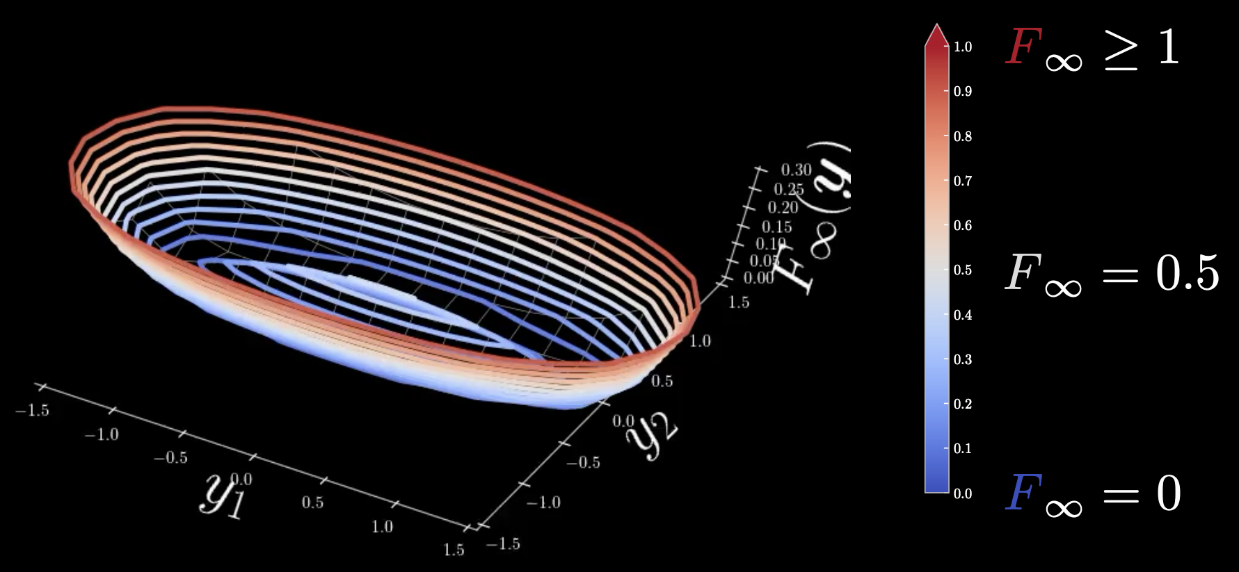
Figure 1: Cold-warm colour map

Cold: $F_\infty = 0$, warm: $F_\infty = 0.5$, hot: $F_\infty \geq 1$

All the regions around the ellipse that is with the manifold ellipse is going to have zero energy but at the centre, there is an infinite zero temperature limit free energy. In order to avoid this, we need to relax the free energy to one without local minima so that it becomes more smooth.

Let’s take a closer look at $y_1=0$, with the following cold-warm map:

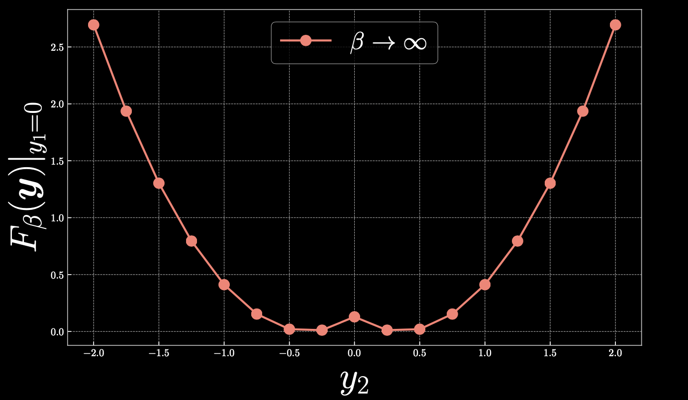
Figure 2

If we take $y_2=0.4$, then $F_\beta(\vect{y})=0$ and as we move linearly away from the point towards the right-hand side, the free energy increases quadratically. Similarly, if we move towards 0, you will end up climbing towards the parabola, creating a peak in the centre.

Relaxed version of free energy

In order to smooth the peak that we previously observed, we need to relax the free energy function such that:

\[F_\beta(\vect{y})\dot{=}-\frac{1}{\beta} \log \frac{1}{\vert\mathcal{Z}\vert}{\int}_\mathcal{Z} \exp[{-\beta}E(\vect{y},z)]\mathrm{d}z\]

where $\beta=(k_B T)^{-1}$ is the inverse temperature, consisting of the Boltzmann constant multiplied by the temperature. If the temperature is very high, $\beta$ is going to be extremely small and if the temperature is cold, then $\beta\rightarrow \infty$.

Simple discrete approximation:

\[\tilde{F}_\beta(\vect{y})=-\frac{1}{\beta} \log \frac{1}{\vert\mathcal{Z}\vert}\underset{z\in\mathcal{Z}}{\sum} \exp[{-\beta}E(y,z)]\Delta z\]

Here, we define $-\frac{1}{\beta} \log \frac{1}{\vert\mathcal{Z}\vert}\underset{z\in\mathcal{Z}}{\sum} \exp[{-\beta}E(\vect{y},z)]$ to be the $\smash{\underset{z}{\text{softmin}}}_\beta[E(\vect{y},z)]$, such that the relaxation of the zero temperature limit free energy becomes the actual-softmin.

Examples:

We will now revisit examples from the previous practicum and see the effects from applying the relaxed version.

Case 1: $\vect{y}’=Y[23]$

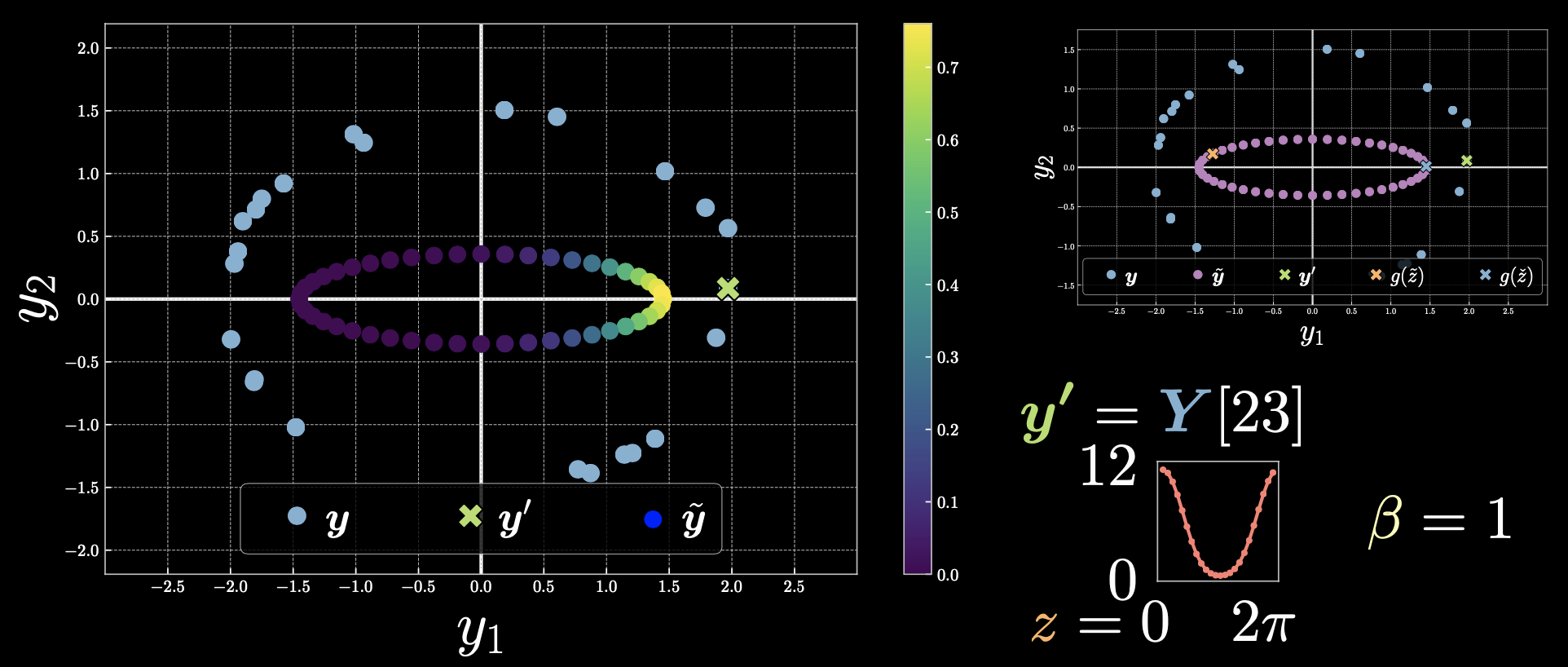
Figure 3

Points that are closer to the point $\vect{y}’$ will have smaller energy, and therefore the exponential will be larger, but for those that are further away the exponential will be zero.

Case 2: $\vect{y}’=Y[10]$

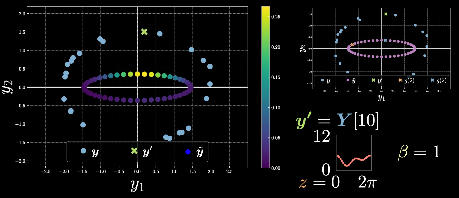
Figure 4

Notice how the colour-bar range changed from the previous example. The upper value here is derived from $\exp[-\beta E(\vect{y},z)]$.

Case 3: $\vect{y}’=(0,0)$

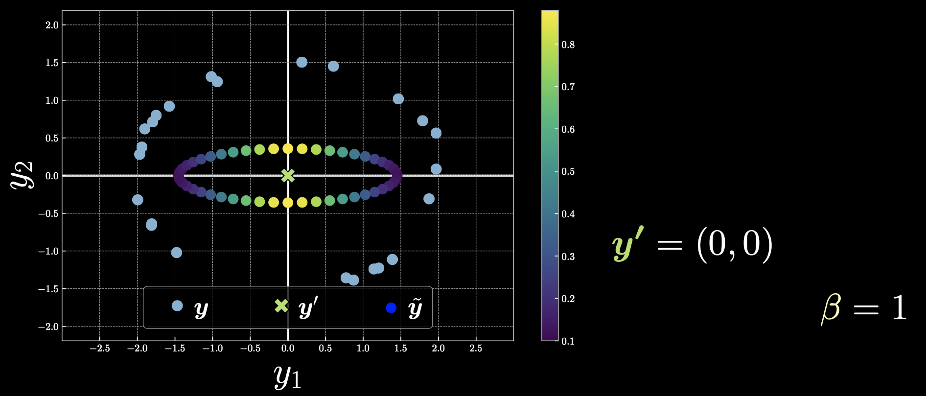
Figure 5

If we choose $\vect{y}’$ to be the origin, then all the points will contribute and the free energy will change symmetrically.

Now, let’s go back to how we can smooth the peak that formed due to the cold energy. If we choose the warmer free energy, we will get the following depiction:

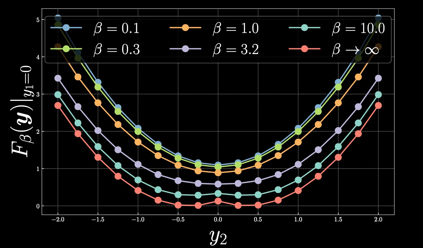
Figure 6

As we increase the temperature by reducing $\beta$, the result is a parabola with a single global minima. As $\beta$ approaches 0, you will end up with the average and recover the MSE.

Nomenclature and PyTorch

Formally, we define the actual-softmax as:

\[\smash{\underset{z}{\text{softmax}}}_\beta[E(y,z)] \doteq \frac{1}{\beta} \log \underset{z\in\mathcal{Z}}{\sum} \exp[{\beta}E(\vect{y},z)] - \frac{1}{\beta} \log{N_z}\]

where $N_z = \vert\mathcal{Z}\vert / \Delta z$. To implement the above function in PyTorch, use torch.logsumexp as below:

\[\smash{\underset{z}{\text{softmax}}}_\beta[E(y,z)] \doteq \frac{1}{\beta} \texttt{torch.logsumexp}({\beta}E(\vect{y},z),\texttt{dim=}z) - \frac{1}{\beta} \log{N_z}\]

Actual-softmin:

\[\smash{\underset{z}{\text{softmin}}}_\beta[E(y,z)] \doteq -\frac{1}{\beta}\log\frac{1}{N_z}\underset{z\in\mathcal{Z}}{\sum}\exp[-{\beta}E(\vect{y},z)]\]

Softmin can be implemented using softmax with 2 negative signs as follows:

\[\smash{\underset{z}{\text{softmin}}}_\beta[E(y,z)] = -\smash{\underset{z}{\text{softmax}}}_\beta[-E(y,z)]\] \[\texttt{torch.softmax}(l(j),\texttt{dim=j}) = \smash{\underset{j}{\text{softargmax}_{\beta=1}}}[l(j)]\]

In technical terms, if free energy is

• hot, it refers to the average.
• warm, it refers to the marginalization of the latent.
• cold, it refers to the minimum value.

Training EBMs

Objective - Finding a well behaved energy function

A loss functional, minimized during learning, is used to measure the quality of the available energy functions. In simple terms, loss functional is a scalar function that tells us how good our energy function is. A distinction should be made between the energy function, which is minimized by the inference process, and the loss functional, which is minimized by the learning process.

\[\mathcal{L}(F(\cdot),Y) = \frac{1}{N} \sum_{n=1}^{N} l(F(\cdot),\vect{y}^{(n)}) \in \R\]

$\mathcal{L}$ is the loss function of the whole dataset that can be expressed as the average of these per sample loss function functionals.

\[l_{\text{energy}}(F(\cdot),\check{\vect{y}}) = F(\check{\vect{y}})\]

where $l_\text{energy}$ is the energy loss functional evaluated in $\vect{y}$ and $\vect{y}$ is the data point on the dataset. $\check{\vect{y}}$ indicates the data points that are to be pushed down. This means the loss functionals should be minimized while training.

The Energy function should be small for data that comes from training distribution but large elsewhere.

\[l_{\text{hinge}}(F(\cdot),\check{\vect{y}},\hat{\vect{y}}) = \big(m - [F(\hat{\vect{y}})-F(\check{\vect{y}})]\big)^{+}\]

where $m$ is the margin and $F(\check{\vect{y}})$ and $F(\hat{\vect{y}})$ are the free energies for “cold” (for correct labels) and “hot” energies (for incorrect labels) respectively.

The model tries to make the difference between two energies to be larger than the margin $m$.

Understand that there is a ReLU function $[\cdot]^{+}$ used on the output of $m - [F(\hat{\vect{y}}) - F(\check{\vect{y}})]$, which means the value of this hinge loss function will always be non-negative. This implies if there are any negative values, they would become $0$ due to this function.

Training will make $F(\hat{\vect{y}})-F(\check{\vect{y}})$ equal or grater than $m$. If the difference becomes greater than $m$, the overall value of $[m - [F(\hat{\vect{y}}) - F(\check{\vect{y}})]]$ becomes negative, the hinge loss becomes $0$. We can also say that we push the energies as long as the difference is less than $m$. However, if the difference becomes greater than the margin $m$, we stop pushing. Hinge Loss Function does not have a smooth margin.

Log loss functional has smooth margin as shown below:

\[l_{\log}(F(\cdot),\check{\vect{y}},\hat{\vect{y}}) = \log(1+\exp[F(\check{\vect{y}})-F(\hat{\vect{y}})])\]

Since, we have an exponential function, this loss has a smoother margin. In other words, it seems like a “soft” version of the hinge loss with an infinite margin.

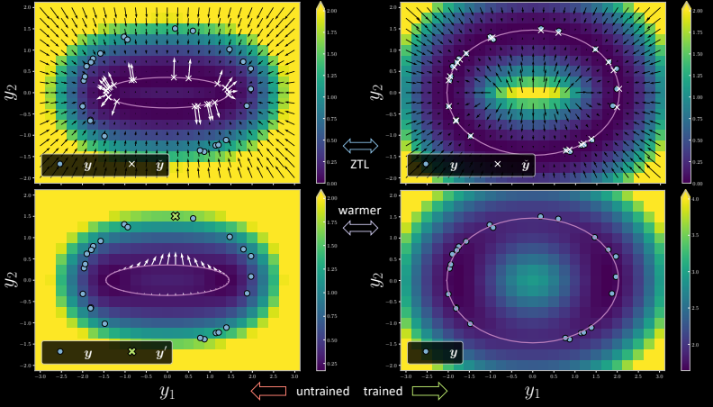
Figure 7

The left hand side is the untrained version where for every training point, there is a corresponding x which is the location on the model manifold closest to the training point as seen in the picture. During training at ZTL (Zero Temperature Limit), the gradient makes the data point on the manifold that is closest to the training point be pushed towards the training point. We can see that after one epoch on the right hand side image, the trained version of the model shows the x points to arrive at the desired location and the energy goes to zero corresponding to the training points (blue points in the figure).

Let’s talk about marginalization now. When the model is trained at ZTL and the temperature is increased, the points were picked individually to be pushed towards the training point. However, in case of marginalization, if we pick one point $\vect{y}$ (the green cross point on the left bottom image), the gradient is just the average of all the arrows pointing towards this particular point $\vect{y}$). This makes all the points that get pulled towards $\vect{y}$, making sure that it does not overfit the training data. Notice how the trained version does not fit over all of the training points.

Let us now see the cross-section of the trained version in this following plot. For the ZTL (${\beta = {\infty}}$), we can see that the free energy has a high peak. As we decrease ${\beta}$, the spike keeps on reducing and we reduce it till we get this smooth parabolic plot in blue, which is the plot in case of marginalization.

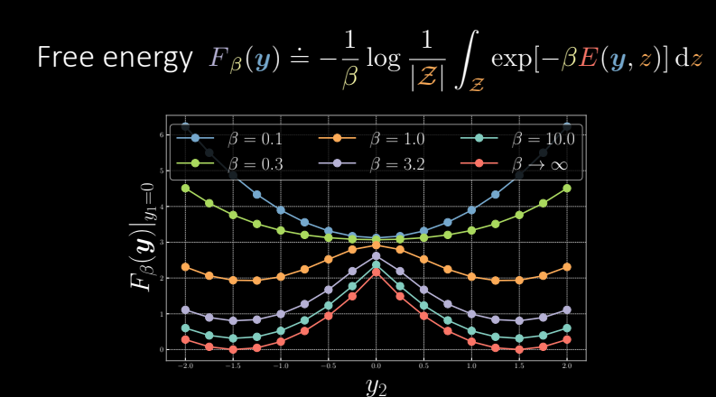
Figure 8 Free energy \[F_{\beta}(\vect{y}) \dot{=} -\frac{1}{\beta}\log\frac{1}{\vert\mathcal{Z}\vert}\int_\mathcal{Z}\exp[-{\beta}E(\vect{y},z)]\mathrm{d}z\]

Now let us move on to Self-Supervised Learning (Conditional case).

Self-supervised learning

A revisit of the training data:

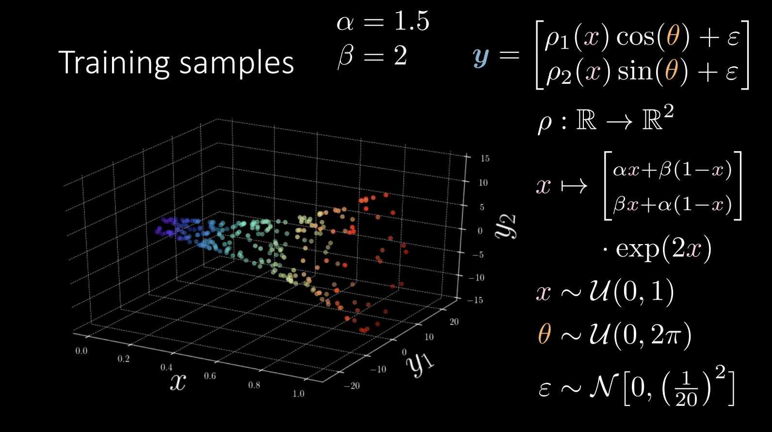
Figure 9

During training, we are trying to learn the shape of the “horn”.

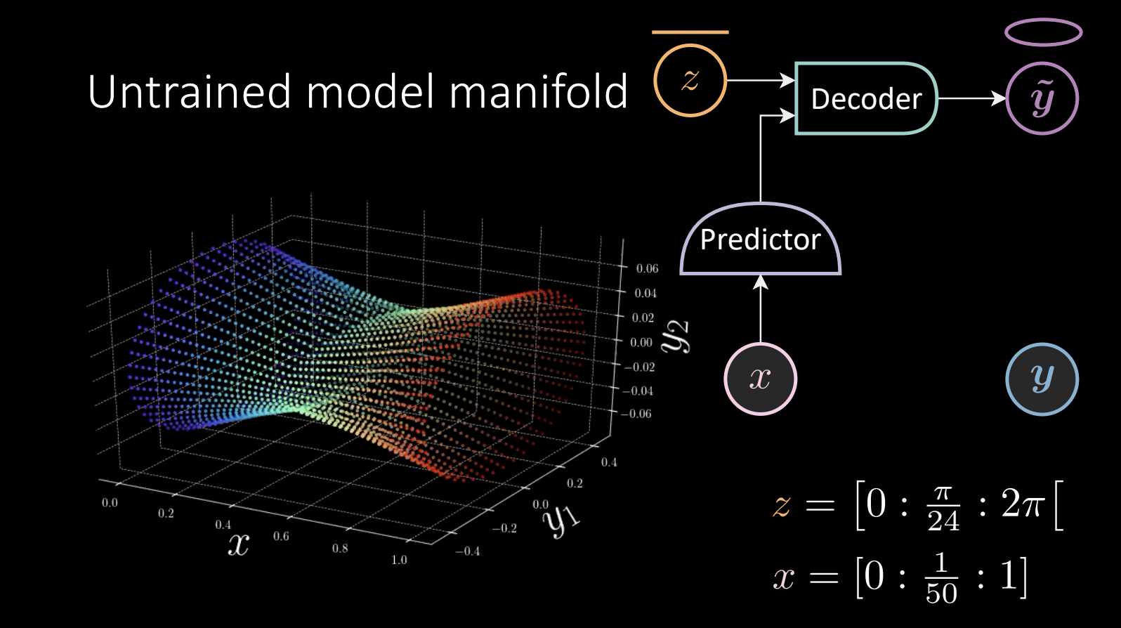
Figure 10 Untrained model manifold \[z = [0:\frac{\pi}{24}: 2\pi[\quad\text{(exclusive of }2\pi)\]

$z$ takes values linearly, and is fed into the decoder to obtain $\tilde{\vect{y}}$, which will go around the ellipse.

\[x = [0:\frac{1}{50} :1]\]

The predictor takes the observed x, and feeds the result into the decoder.

We perform zero temperature free energy training, which gives a result:

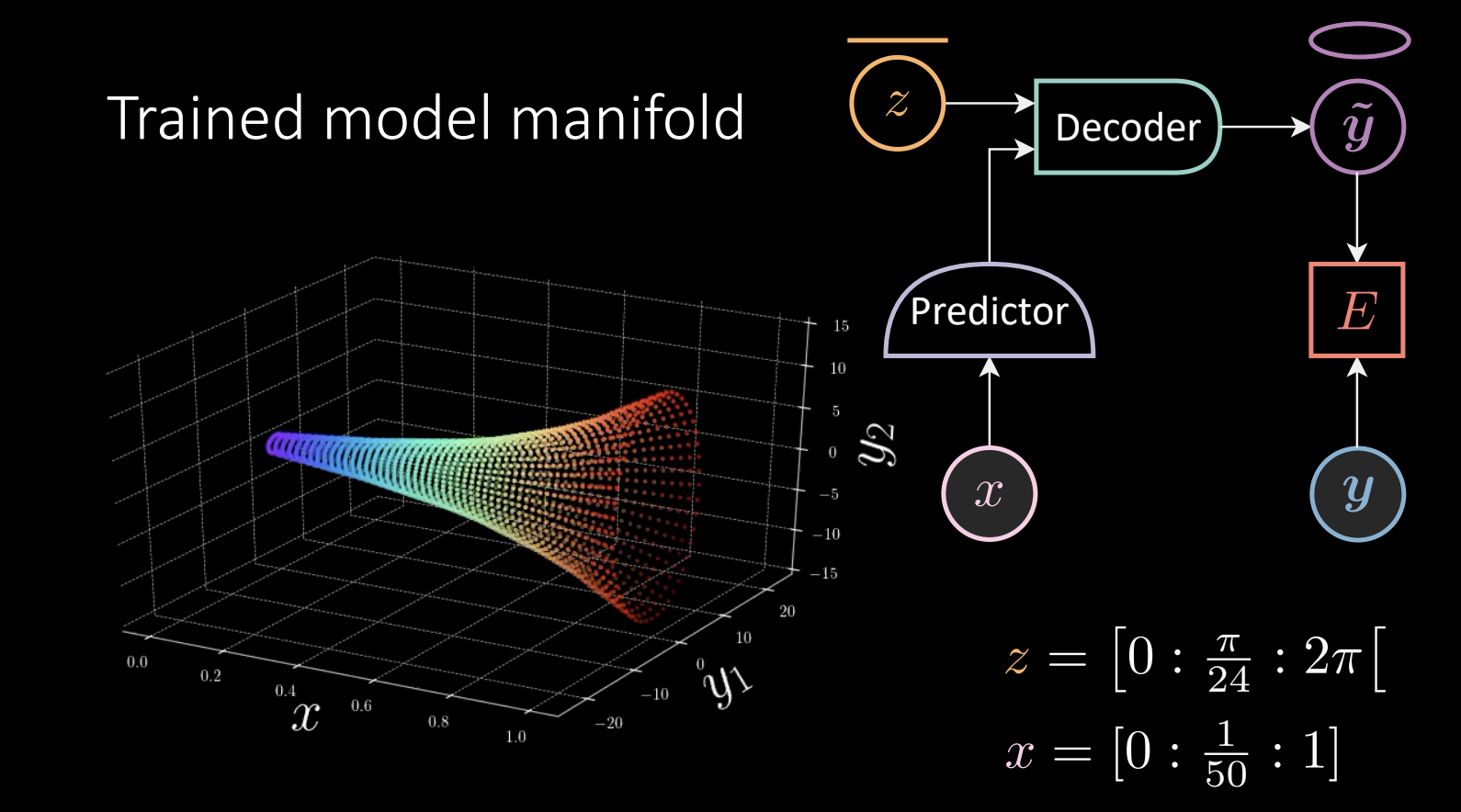
Figure 11 Untrained model manifold

Given the “horn”, we take one point $\vect{y}$, find the closest point on the manifold and pull it towards $\vect{y}$.

In this case, the energy function is defined as

\[E(x,\vect{y},z) = [\vect{y}_{1} - f_{1}(x)g_{1}(z)]^{2} + [\vect{y}_{2} -f_{2}(x)g_{2}(z)]^{2}\]

where

\[f,g:\mathbb{R} \rightarrow \mathbb{R}^{2}\] \[\begin{array}{l} x \stackrel{f}{\mapsto} x \stackrel{\mathrm{L}^{+}}{\rightarrow} 8 \stackrel{\mathrm{L}^{+}}{\rightarrow} 8 \stackrel{\mathrm{L}}{\rightarrow} 2 \\ z \stackrel{g}{\mapsto}[\cos (z) \quad \sin (z)]^{\top} \end{array}\]

The component of $g$ will be scaled by output of $f$.

The example data takes no time to train, but how do we move forward to generalize it?

\[\begin{array}{l} f: \mathbb{R} \rightarrow \mathbb{R}^{\operatorname{dim}(f)} \\ g: \mathbb{R}^{\operatorname{dim}(f)} \times \mathbb{R} \rightarrow \mathbb{R}^{2} \end{array} \\ E(x, \vect{y}, z)=\left[\vect{y}_{1}-g_{1}(f(x), z)\right]^{2}+\left[\vect{y}_{2}-g_{2}(f(x), z)\right]^{2}\]

In this case the $g$ function takes $f$ and $z$, and $g$ can be a neural net. This time, the model has to learn that $\vect{y}$ moves around in circle, which is the $\sin$ and $\cos$ part we take for granted before.

Another issue is to determine the dimension of latent variable $z$.

\[\begin{array}{l} f: \mathbb{R} \rightarrow \mathbb{R}^{\operatorname{dim}(f)} \\ g: \mathbb{R}^{\operatorname{dim}(f)} \times \mathbb{R}^{\operatorname{dim}(z)} \rightarrow \mathbb{R}^{2} \end{array}\\ E(x, \vect{y}, z)=\left[\vect{y}_{1}-g_{1}(f(x), z)\right]^{2}+\left[\vect{y}_{2}-g_{2}(f(x), z)\right]^{2}\]

Since a high dimension latent will lead to overfitting. We need to regularize $z$. Otherwise, the model will memorize all the points, causing the energy to be zero across the space.

---

📝 Anu-Ujin Gerelt-Od, Sunidhi Gupta, Bichen Kou, Binfeng Xu
31 Oct 2020