RNNs, GRUs, LSTMs, Attention, Seq2Seq, and Memory Networks

Deep Learning Architectures

In deep learning, there are different modules to realize different functions. Expertise in deep learning involves designing architectures to complete particular tasks. Similar to writing programs with algorithms to give instructions to a computer in earlier days, deep learning reduces a complex function into a graph of functional modules (possibly dynamic), the functions of which are finalized by learning.

As with what we saw with convolutional networks, network architecture is important.

Recurrent Networks

In a Convolutional Neural Network, the graph or interconnections between the modules cannot have loops. There exists at least a partial order among the modules such that the inputs are available when we compute the outputs.

As shown in Figure 1, there are loops in Recurrent Neural Networks.

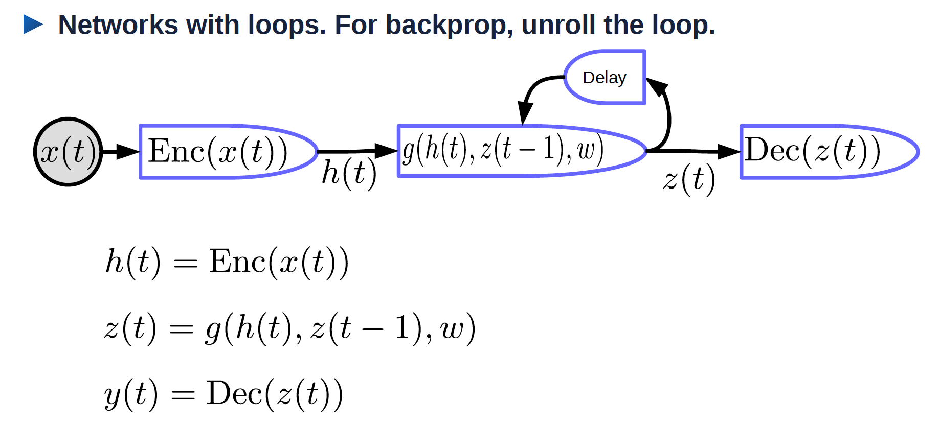
Figure 1. Recurrent Neural Network with roll

• $x(t)$ : input that varies across time
• $\text{Enc}(x(t))$: encoder that generates a representation of input
• $h(t)$: a representation of the input
• $w$: trainable parameters
• $z(t-1)$: previous hidden state, which is the output of the previous time step
• $z(t)$: current hidden state
• $g$: function that can be a complicated neural network; one of the inputs is $z(t-1)$ which is the output of the previous time step
• $\text{Dec}(z(t))$: decoder that generates an output

Recurrent Networks: Unroll the loop

Unroll the loop in time. The input is a sequence $x_1, x_2, \cdots, x_T$.

"
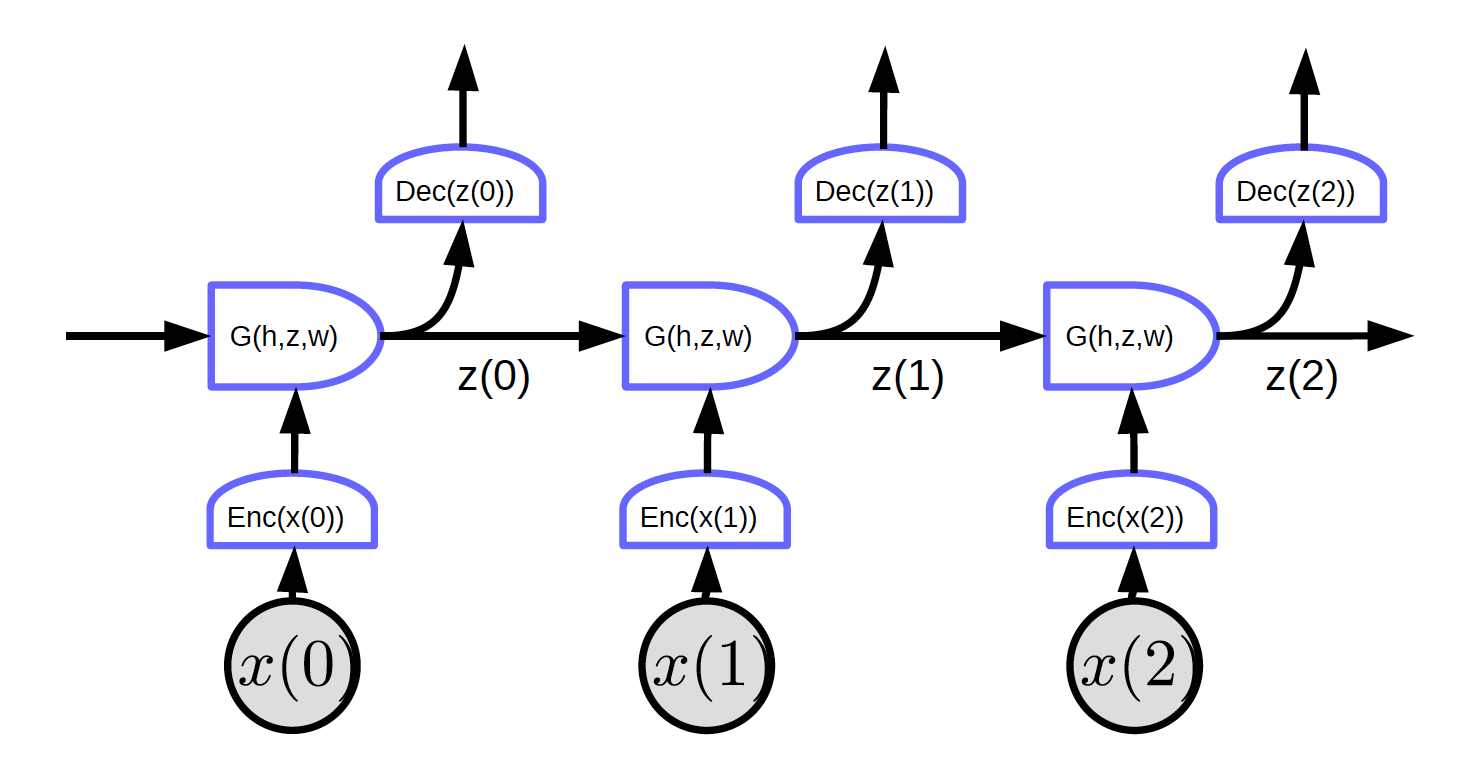
Figure 2. Recurrent Networks with unrolled loop

In Figure 2, the input is $x_1, x_2, x_3$.

At time t=0, the input $x(0)$ is passed to the encoder and it generates the representation $h(x(0)) = \text{Enc}(x(0))$ and then passes it to G to generate hidden state $z(0) = G(h_0, z’, w)$. At $t = 0$, $z’$ in $G$ can be initialized as $0$ or randomly initialized. $z(0)$ is passed to decoder to generate an output and also to the next time step.

As there are no loops in this network, and we can implement backpropagation.

Figure 2 shows a regular network with one particular characteristic: every block shares the same weights. Three encoders, decoders and G functions have same weights respectively across different time steps.

BPTT: Backprop through time. Unfortunately, BPTT doesn’t work so well in the naive form of RNN.

Problems with RNNs:

1. Vanishing gradients
   • In a long sequence, the gradients get multiplied by the weight matrix (transpose) at every time step. If there are small values in the weight matrix, the norm of gradients get smaller and smaller exponentially.
2. Exploding gradients
   • If we have a large weight matrix and the non-linearity in the recurrent layer is not saturating, the gradients will explode. The weights will diverge at the update step. We may have to use a tiny learning rate for the gradient descent to work.

One reason to use RNNs is for the advantage of remembering information in the past. However, it could fail to memorize the information long ago in a simple RNN without tricks.

An example that has vanishing gradient problem:

The input is the characters from a C Program. The system will tell whether it is a syntactically correct program. A syntactically correct program should have a valid number of braces and parentheses. Thus, the network should remember how many open parentheses and braces there are to check, and whether we have closed them all. The network has to store such information in hidden states like a counter. However, because of vanishing gradients, it will fail to preserve such information in a long program.

RNN Tricks

• clipping gradients: (avoid exploding gradients) Squash the gradients when they get too large.
• Initialization (start in right ballpark avoids exploding/vanishing) Initialize the weight matrices to preserve the norm to some extent. For example, orthogonal initialization initializes the weight matrix as a random orthogonal matrix.

Multiplicative Modules

In multiplicative modules rather than only computing a weighted sum of inputs, we compute products of inputs and then compute weighted sum of that.

Suppose $x \in {R}^{n\times1}$, $W \in {R}^{m \times n}$, $U \in {R}^{m \times n \times d}$ and $z \in {R}^{d\times1}$. Here U is a tensor.

where $s_i = w_{i}^\top x = \sum_j w_{ij}x_j$.

The output of the system is a classic weighted sum of inputs and weights. Weights themselves are also weighted sums of weights and inputs.

Hypernetwork architecture: weights are computed by another network.

Attention

$x_1$ and $x_2$ are vectors, $w_1$ and $w_2$ are scalars after softmax where $w_1 + w_2 = 1$, and $w_1$ and $w_2$ are between 0 and 1.

$w_1x_1 + w_2x_2$ is a weighted sum of $x_1$ and $x_2$ weighted by coefficients $w_1$ and $w_2$.

By changing the relative size of $w_1$ and $w_2$, we can switch the output of $w_1x_1 + w_2x_2$ to $x_1$ or $x_2$ or some linear combinations of $x_1$ and $x_2$.

The inputs can have multiple $x$ vectors (more than $x_1$ and $x_2$). The system will choose an appropriate combination, the choice of which is determined by another variable z. An attention mechanism allows the neural network to focus its attention on particular input(s) and ignore the others.

Attention is increasingly important in NLP systems that use transformer architectures or other types of attention.

The weights are data independent because z is data independent.

Gated Recurrent Units (GRU)

As mentioned above, RNN suffers from vanishing/exploding gradients and can’t remember states for very long. GRU, Cho, 2014, is an application of multiplicative modules that attempts to solve these problems. It’s an example of recurrent net with memory (another is LSTM). The structure of A GRU unit is shown below:

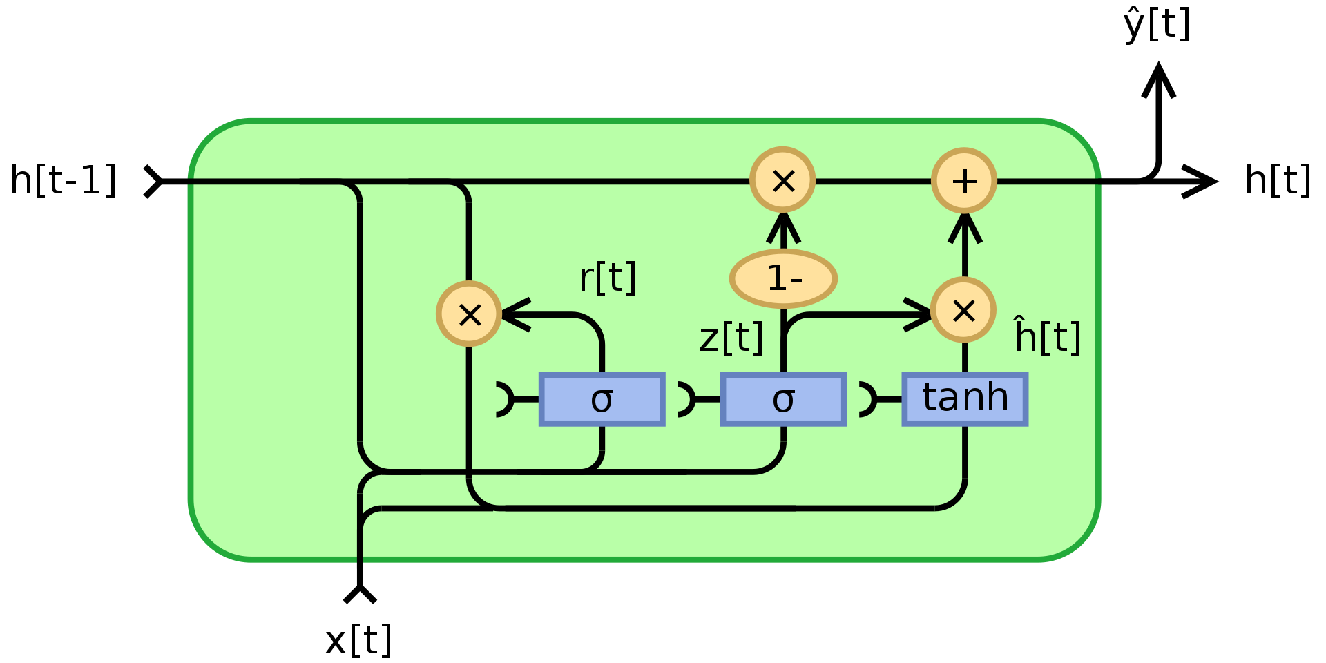
Figure 3. Gated Recurrent Unit

where $\odot$ denotes element-wise multiplication(Hadamard product), $x_t$ is the input vector, $h_t$ is the output vector, $z_t$ is the update gate vector, $r_t$ is the reset gate vector, $\phi_h$ is a hyperbolic tanh, and $W$,$U$,$b$ are learnable parameters.

To be specific, $z_t$ is a gating vector that determines how much of the past information should be passed along to the future. It applies a sigmoid function to the sum of two linear layers and a bias over the input $x_t$ and the previous state $h_{t-1}$. $z_t$ contains coefficients between 0 and 1 as a result of applying sigmoid. The final output state $h_t$ is a convex combination of $h_{t-1}$ and $\phi_h(W_hx_t + U_h(r_t\odot h_{t-1}) + b_h)$ via $z_t$. If the coefficient is 1, the current unit output is just a copy of the previous state and ignores the input (which is the default behaviour). If it is less than one, then it takes into account some new information from the input.

The reset gate $r_t$ is used to decide how much of the past information to forget. In the new memory content $\phi_h(W_hx_t + U_h(r_t\odot h_{t-1}) + b_h)$, if the coefficient in $r_t$ is 0, then it stores none of the information from the past. If at the same time $z_t$ is 0, then the system is completely reset since $h_t$ would only look at the input.

LSTM (Long Short-Term Memory)

GRU is actually a simplified version of LSTM which came out much earlier, Hochreiter, Schmidhuber, 1997. By building up memory cells to preserve past information, LSTMs also aim to solve long term memory loss issues in RNNs. The structure of LSTMs is shown below:

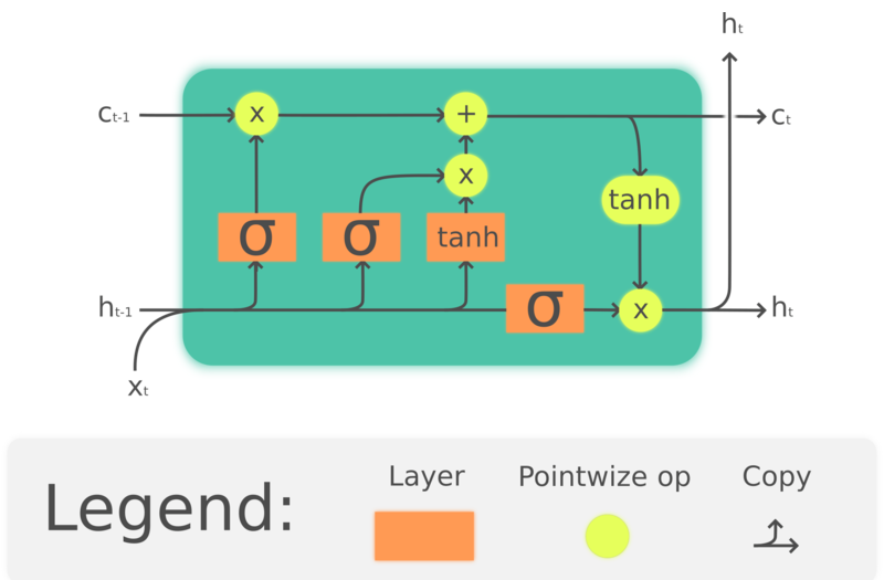
Figure 4. LSTM

where $\odot$ denotes element-wise multiplication, $x_t\in\mathbb{R}^a$ is an input vector to the LSTM unit, $f_t\in\mathbb{R}^h$ is the forget gate’s activation vector, $i_t\in\mathbb{R}^h$ is the input/update gate’s activation vector, $o_t\in\mathbb{R}^h$ is the output gate’s activation vector, $h_t\in\mathbb{R}^h$ is the hidden state vector (also known as output), $c_t\in\mathbb{R}^h$ is the cell state vector.

An LSTM unit uses a cell state $c_t$ to convey the information through the unit. It regulates how information is preserved or removed from the cell state through structures called gates. The forget gate $f_t$ decides how much information we want to keep from the previous cell state $c_{t-1}$ by looking at the current input and previous hidden state, and produces a number between 0 and 1 as the coefficient of $c_{t-1}$. $\tanh(W_cx_t + U_ch_{t-1} + b_c)$ computes a new candidate to update the cell state, and like the forget gate, the input gate $i_t$ decides how much of the update to be applied. Finally, the output $h_t$ will be based on the cell state $c_t$, but will be put through a $\tanh$ then filtered by the output gate $o_t$.

Though LSTMs are widely used in NLP, their popularity is decreasing. For example, speech recognition is moving towards using temporal CNN, and NLP is moving towards using transformers.

Sequence to Sequence Model

The approach proposed by Sutskever NIPS 2014 is the first neural machine translation system to have comparable performance to classic approaches. It uses an encoder-decoder architecture where both the encoder and decoder are multi-layered LSTMs.

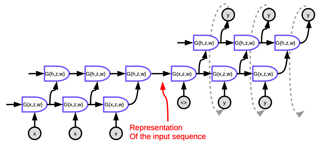
Figure 5. Seq2Seq

Each cell in the figure is an LSTM. For the encoder (the part on the left), the number of time steps equals the length of the sentence to be translated. At each step, there is a stack of LSTMs (four layers in the paper) where the hidden state of the previous LSTM is fed into the next one. The last layer of the last time step outputs a vector that represents the meaning of the entire sentence, which is then fed into another multi-layer LSTM (the decoder), that produces words in the target language. In the decoder, the text is generated in a sequential fashion. Each step produces one word, which is fed as an input to the next time step.

This architecture is not satisfying in two ways: First, the entire meaning of the sentence has to be squeezed into the hidden state between the encoder and decoder. Second, LSTMs actually do not preserve information for more than about 20 words. The fix for these issues is called a Bi-LSTM, which runs two LSTMs in opposite directions. In a Bi-LSTM the meaning is encoded in two vectors, one generated by running LSTM from left to right, and another from right to left. This allows doubling the length of the sentence without losing too much information.

Seq2seq with Attention

The success of the approach above was short-lived. Another paper by Bahdanau, Cho, Bengio suggested that instead of having a gigantic network that squeezes the meaning of the entire sentence into one vector, it would make more sense if at every time step we only focus the attention on the relevant locations in the original language with equivalent meaning, i.e. the attention mechanism.

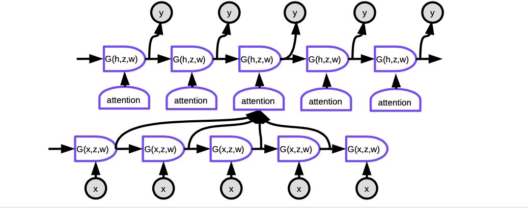
Figure 6. Seq2Seq with Attention

In Attention, to produce the current word at each time step, we first need to decide which hidden representations of words in the input sentence to focus on. Essentially, a network will learn to score how well each encoded input matches the current output of the decoder. These scores are normalized by a softmax, then the coefficients are used to compute a weighted sum of the hidden states in the encoder at different time steps. By adjusting the weights, the system can adjust the area of inputs to focus on. The magic of this mechanism is that the network used to compute the coefficients can be trained through backpropagation. There is no need to build them by hand!

Attention mechanisms completely transformed neural machine translation. Later, Google published a paper Attention Is All You Need, and they put forward transformer, where each layer and group of neurons is implementing attention.

Memory network

Memory networks stem from work at Facebook that was started by Antoine Bordes in 2014 and Sainbayar Sukhbaatar in 2015.

The idea of a memory network is that there are two important parts in your brain: one is the cortex, which is where you have long term memory. There is a separate chunk of neurons called the hippocampus which sends wires to nearly everywhere in the cortex. The hippocampus is thought to be used for short term memory, remembering things for a relatively short period of time. The prevalent theory is that when you sleep, there is a lot of information transferred from the hippocampus to the cortex to be solidified in long term memory since the hippocampus has limited capacity.

For a memory network, there is an input to the network, $x$ (think of it as an address of the memory), and compare this $x$ with vectors $k_1, k_2, k_3, \cdots$ (“keys”) through a dot product. Put them through a softmax, what you get are an array of numbers which sum to one. And there are a set of other vectors $v_1, v_2, v_3, \cdots$ (“values”). Multiply these vectors by the scalers from softmax and sum these vectors up (note the resemblance to the attention mechanism) gives you the result.

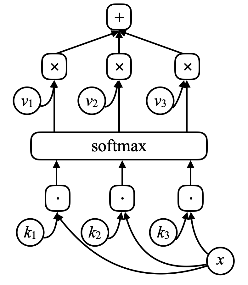
Figure 7. Memory Network

If one of the keys (e.g. $k_i$) exactly matches $x$, then the coefficient associated with this key will be very close to one. So the output of the system will essentially be $v_i$.

This is addressable associative memory. Associative memory is that if your input matches a key, you get that value. And this is just a soft differentiable version of it, which allows you to backpropagate and change the vectors through gradient descent.

What the authors did was tell a story to a system by giving it a sequence of sentences. The sentences are encoded into vectors by running them through a neural net that has not been pretrained. The sentences are returned to the memory of this type. When you ask a question to the system, you encode the question and put it as the input of a neural net, the neural net produces an $x$ to the memory, and the memory returns a value.

This value, together with the previous state of the network, is used to re-access the memory. And you train this entire network to produce an answer to your question. After extensive training, this model actually learns to store stories and answer questions.

In memory network, there is a neural net that takes an input and then produces an address for the memory, gets the value back to the network, keeps going, and eventually produces an output. This is very much like computer since there is a CPU and an external memory to read and write.

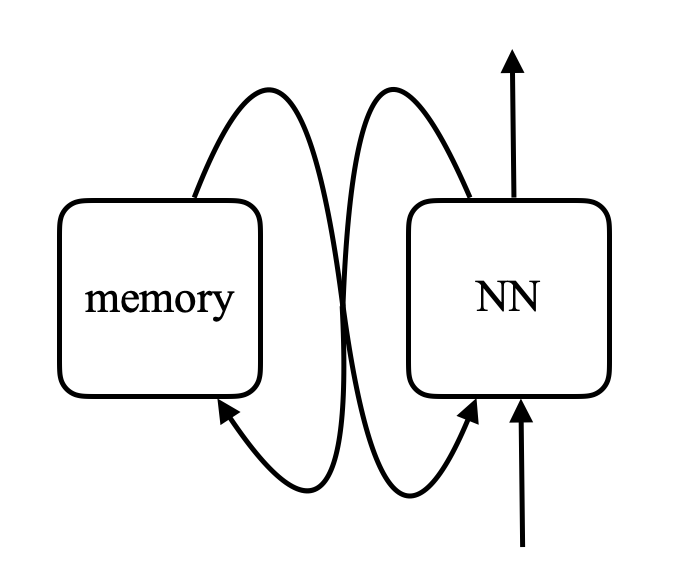
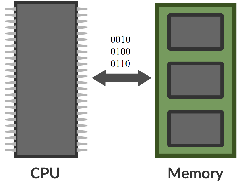
Figure 8. Comparision between memory network and computer (Photo by Khan Acadamy)

There are people who imagine that you can actually build differentiable computers out of this. One example is the Neural Turing Machine from DeepMind, which was made public three days after Facebook’s paper was published on arXiv.

The idea is to compare inputs to keys, generate coefficients, and produce values - which is basically what a transformer is. A transformer is basically a neural net in which every group of neurons is one of these networks.