Graph Convolutional Networks II

Spectral Graph ConvNets (GCNs)

In the previous section we discussed Graph Spectral Theory, one of the two ways to define convolution for graphs, which we can now use to define Spectral GCNs.

Vanilla Spectral GCN

We define a graph spectral convolutional layer such that given layer $h^l$, the activation of the next layer is:

where $\eta$ represents a nonlinear activation and $w^l$ is a spatial filter. The RHS of the equation is equivalent to $\eta(\hat{w}^l(\Delta)h^l)$ where $\hat{w}^l$ represents a spectral filter and $\Delta$ is the Laplacian. We can further decompose the RHS of the equation into $\eta(\boldsymbol{\phi} \hat{w}^l(\Lambda)\boldsymbol{\phi^\top} h^l)$, where $\boldsymbol{\phi}$ is the Fourier matrix and $\Lambda$ is the eigenvalues. This yields the final activation equation as below.

The objective is to learn the spectral filter $\hat{w}^l(\lambda)$ using backpropagation instead of hand crafting.

This technique was the first spectral technique used for ConvNets, but it has a few limitations:

• No guarantee of spatial localization of filters
• Need to learn $O(n)$ parameters per layer ($\hat{w}(\lambda_1)$ to $\hat{w}(\lambda_n)$)
• Learning rate is $O(n^2$) because $\boldsymbol{\phi}$ is a dense matrix

SplineGCNs

SplineGCNs involve computing smooth spectral filters to get localized spatial filters. The connection between smoothness in frequency domain and localization in space is based on Parseval’s Identity (also Heisenberg uncertainty principle): smaller derivative of spectral filter (smoother function) $\Leftrightarrow$ smaller variance of spatial filter (localization).

How do we get a smooth spectral filter? We decompose the spectral filter to be a linear combination of $K$ smooth kernels $\boldsymbol{B}$ (splines) so that $\hat{w}^l(\Lambda)=diag(\boldsymbol{B}w^l)$. The activation equation the is as the following.

Now, we only have $O(1)$ parameters (constant $K$) per layer to be learned through backpropagation. However, the learning complexity is still $O(n^2)$.

LapGCNs

How do we learn in linear time $O(n)$ (w.r.t. graph size $n$)? The $O(n^2)$ complexity is a direct result of using Laplacian eigenvectors. We need to avoid eigen-decomposition, which can be achieved by directly learning a function of the Laplacian. The spectral function will be a monomial of the Laplacian as shown here.

One nice feature is that filters are localized in exactly k-hop supports.

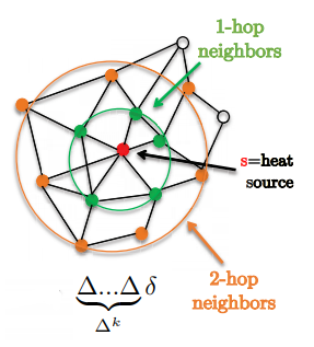
Figure 1: Demonstrates 1-hop and 2-hop neighbourhoods

We replace the expression $\Delta^kh$ with $X_k$, a recursive equation defined as,

Complexity is now $O(E.K)=O(n)$ for sparse (real-world) graphs. We can reshape $X_k$ into $\bar{X}$ to form a linear operation. We now have the following activation equation.

Note: Since no Laplacian eigen-decomposition is used, all operations are in the spatial (not spectral) domain, so calling them Spectral GCNs may be misguided. Further, another drawback of LapGCNs is that convolutional layers involve sparse linear operations, which GPU’s are not fully optimized for.

We now have resolved the 3 limitations of Vanilla GCNs through localized filters (in $K$-hop support), $O(1)$ parameters per layer and $O(n)$ learning complexity. However, the limitation of LapGCNs is that monomial basis ($\Delta^0,\Delta^1,\ldots$) used is unstable for optimization because it is not orthogonal (changing one coefficient changes the function approximation).

ChebNets

To resolve the issue of unstable basis we can use any orthonormal basis, but it must have a recursive equation to ensure linear complexity. For ChebNets we use Chebyshev polynomials, and as in a LapGCN we represent the expression $T_k(\Delta)h$ (Chebyshev function applied to $h$) by $X_k$, a recursive equation defined as,

Now we have stability under coefficient perturbation.

ChebNets are GCNs that can be used for any arbitrary graph domain, but the limitation is that they are isotropic. Standard ConvNets produce anisotropic filters because Euclidean grids have direction, while Spectral GCNs compute isotropic filters since graphs have no notion of direction (up, down, left, right).

We can extend ChebNets to multiple graphs using a 2D spectral filter. This may be useful, for example, in recommender systems where we have movie graphs and user graphs. Multi-graph ChebNets have the activation equation as below.

CayleyNets

ChebNets are unstable to produce filters (localize) with frequency bands of interest (graph communities). In CayleyNets, we instead use as our orthonormal basis Cayley rationals.

CayleyNets have the same properties as ChebNets (are isotropic), but they are localized in frequency (with spectral zoom) and provide a richer class of filters (for the same order $K$).

Spatial Graph ConvNets

Template Matching

To understand Spatial Graph ConvNets, we go back to the Template Matching definition of ConvNets.

The main issue when we perform Template Matching for graphs is the lack of node ordering or positioning for the template. All we have are the indices of nodes, which isn’t enough to match information between them. How do we design template matching to be invariant to node re-parametrisation? That is, if we have a graph and one of the nodes had an arbitrary index, say 6, this index could’ve been 122 as well. So it’s essential to be able to perform template matching independent to the index of the node.

The simplest way to do this is by having only one template vector $w^l$, instead of having $w_{j1}$,$w_{j2}$, $w_{j3}$ or so on. So we match this vector $w^l$ with all other features on our graph. Most Graph Neural Networks today use this property.

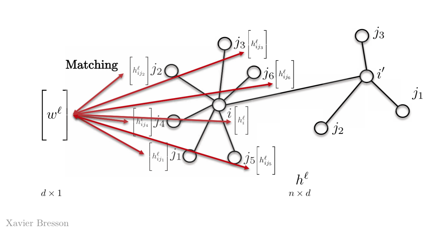
Figure 2: Template Matching using a template vector

Mathematically, for one feature we have,

where, $w^l$ is the template vector at layer $l$ of dimensions $d \times 1$ and $h_{ij}^l$ is the vector at node j with $d \times 1$ which will result in a scalar quantity $h_{i}^{l+1}$ at node $i$.

for more($d$) features,

where, $\boldsymbol{W}^l$ is of the dimensionality $d \times d$ and $h_{i}^{l+1}$ is $d \times 1$

for a vectoral representation,

where, $\boldsymbol{A}$ is the adjacency matrix of dimensions $n \times n$, $h^l$ is the activation function at the layer $l$ with dimensions $n \times d$.

Based on this definition of Template Matching we can define two types of Spatial GSNs – Isotropic GCNs and Anisotropic GCNs.

Isotropic GCNs

Vanilla Spatial GCNs

It has the same definition as before, but we add the Diagonal matrix in the equation, in such a way that we find the mean value of the neighbourhood.

Matrix representation being,

where, $\boldsymbol{A}$ has the dimensions $n \times n$, $h^{l}$ has dimensions $n \times d$ and $W^{l}$ has $d \times d$, which results in a $n \times d$ $h^{l+1}$ matrix.

And the vectorial representation being,

where, $h_{i}^{l+1}$ has the dimensions of $d \times 1$

The vectorial representation is responsible for handling the absence of node ordering, which is invariant of node re-parametrisation. That is, adding on the previous example, if the node has an in 6 and is changed to 122, this won’t change anything in the computation of the activation function of the next layer $h^{l+1}$.

We can also deal with neighbourhood of different sizes. That is we can have a neighbourhood of 4 nodes or 10 nodes, it wouldn’t change anything.

We are given the local reception field by design, that is, with Graph Neural Networks we only have to consider the neighbours.

We have weight sharing, that is, we the same $\boldsymbol{W}^{l}$ matrix for all features no matter the position of the graph, which is a Convolution property.

This formulation is also independent of the graph size, since all operations are done locally.

Since it is an isotropic model, the neighbours will have the same $\boldsymbol{W}^{l}$ matrix.

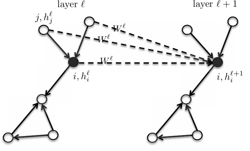
Figure 3: Isotropic model

So, the activation of the next layer $h_{i}^{l+1}$ is a function of the activation of the previous layer $h_{i}^{l}$ at node $i$ and the neighbourhood of $i$. When we change the function, we get an entire family of graphs.

ChebNets and Vanilla Spatial GCNs

The above defined Vanilla Spatial GCN is a simplification of ChebNets. We can truncate the expansion of ChebNet by using the first two Chebyshev functions to end up with,

GraphSage

If the Adjacency matrix $\boldsymbol{A}_{ij} = 1$ for the edges in Vanilla Spatial GCNs, we get,

For this equation, we give the central/core vertex $i$ and it’s neighbourhood the same template weight $\boldsymbol{W}^{l}$. We can differentiate this by giving the central node $\boldsymbol{W}_{1}^{l}$, and having a different template node $\boldsymbol{W}_{2}^{l}$ for the one-hot neighbourhood. This will improve the performance of the GNNs by a substantial amount. This model is still considered to be Isotropic in nature, since the neighbours have the same weight.

where, $\boldsymbol{W}_{1}^{l}$ and $\boldsymbol{W}_{2}^{l}$ are of dimension $d \times d$; $h_{i}^{l}$ and $h_{j}^{l}$ are of the dimension $d \times 1$.

In this equation, we can find the summation or maximum of $\boldsymbol{W}_{2}^{l} h_{j}^{l}$ or the Long-Short Term Memory of $h_{j}^{l}$, instead of the mean.

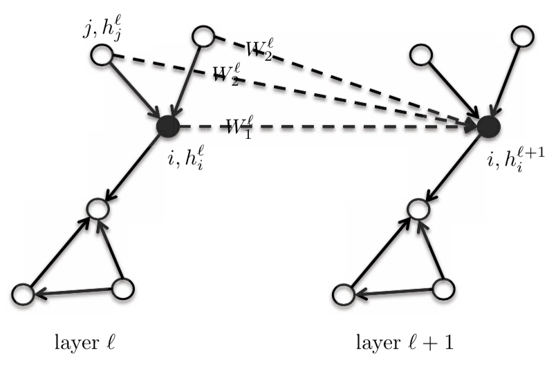
Figure 4: GraphSage

Graph Isomorphism Networks (GIN)

An architecture that can differentiate graphs that are not isomorphic. Isomorphism is the measure of equivalence between graphs. In the figure below, the two graphs are considered isomorphic to each other. Isomorphic graphs will be treated in a similar way and non-isomorphic graphs will be treated differently.

GIN is an isotropic GCN.

where, $\texttt{BN}$ stands for Batch Normalization.

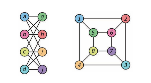
Figure 5: Examples of two isomorphic graphs

Anisotropic GCNs

Standard CNNs have the ability to produce anisotropic filters — ones that favour certain directions. This is because the directional structure is based on up, down, left, and right. However, the GCNs described above have no notion of direction, and thus can only produce isotropic filters. Anisotropy can be introduced naturally, with edge features. For instance, molecules can have single, double, and triple bonds. Graphically, it is introduced weighting different neighbours differently.

MoNets

MoNets use the degree of the graph to learn the parameters of a Gaussian Mixture Model (GMM).

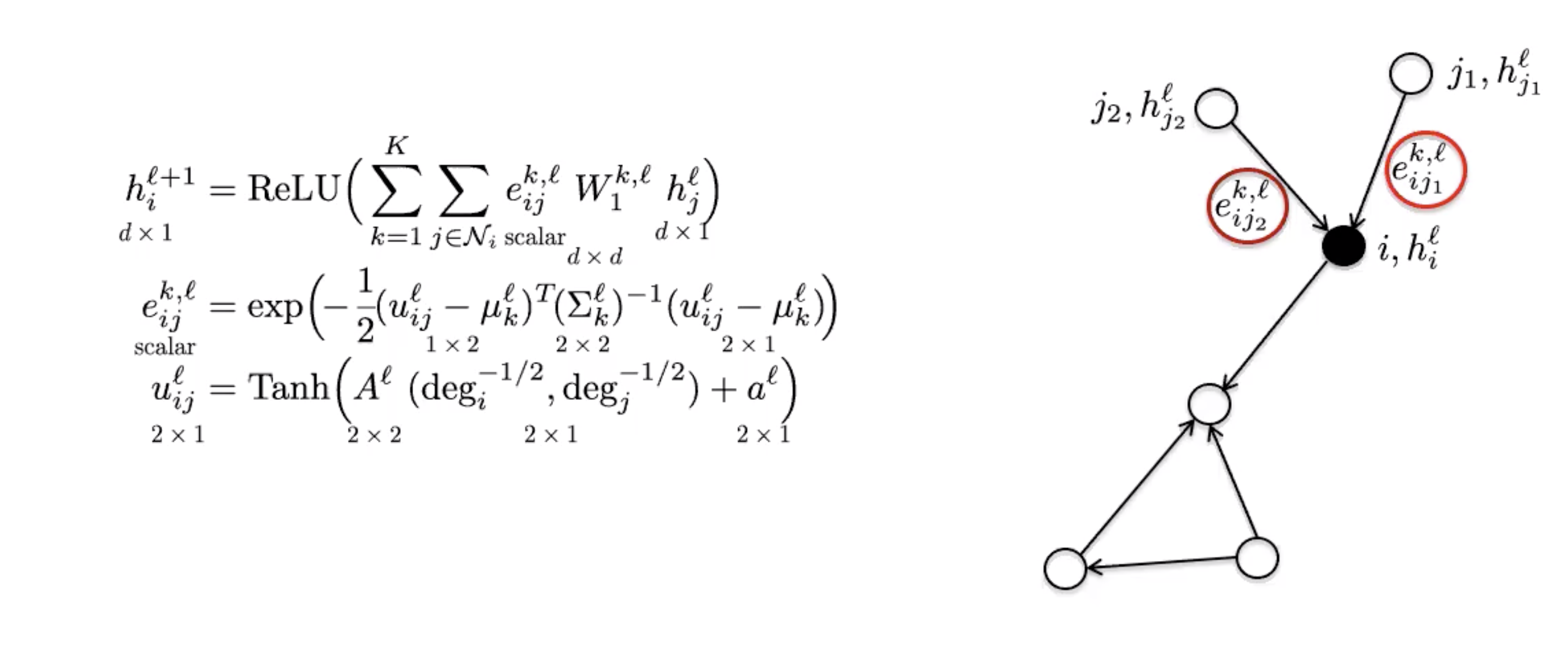
Figure 6: MoNet

Graph Attention Networks (GAT)

GAT uses the attention mechanism to introduce anisotropy in the neighbourhood aggregation function.

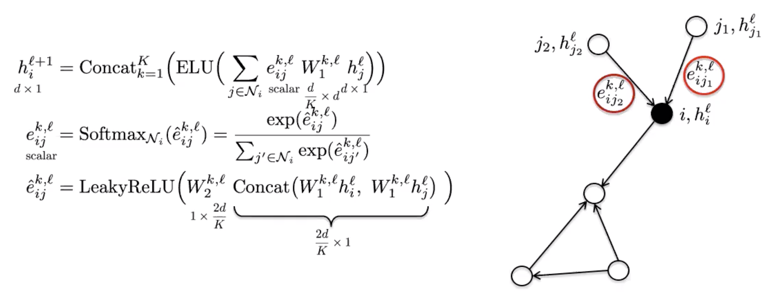
Figure 7: GAT

Gated Graph ConvNets

These use a simple edge gating mechanism, which can be seen as a softer attention process as the sparse attention mechanism used in GATs.

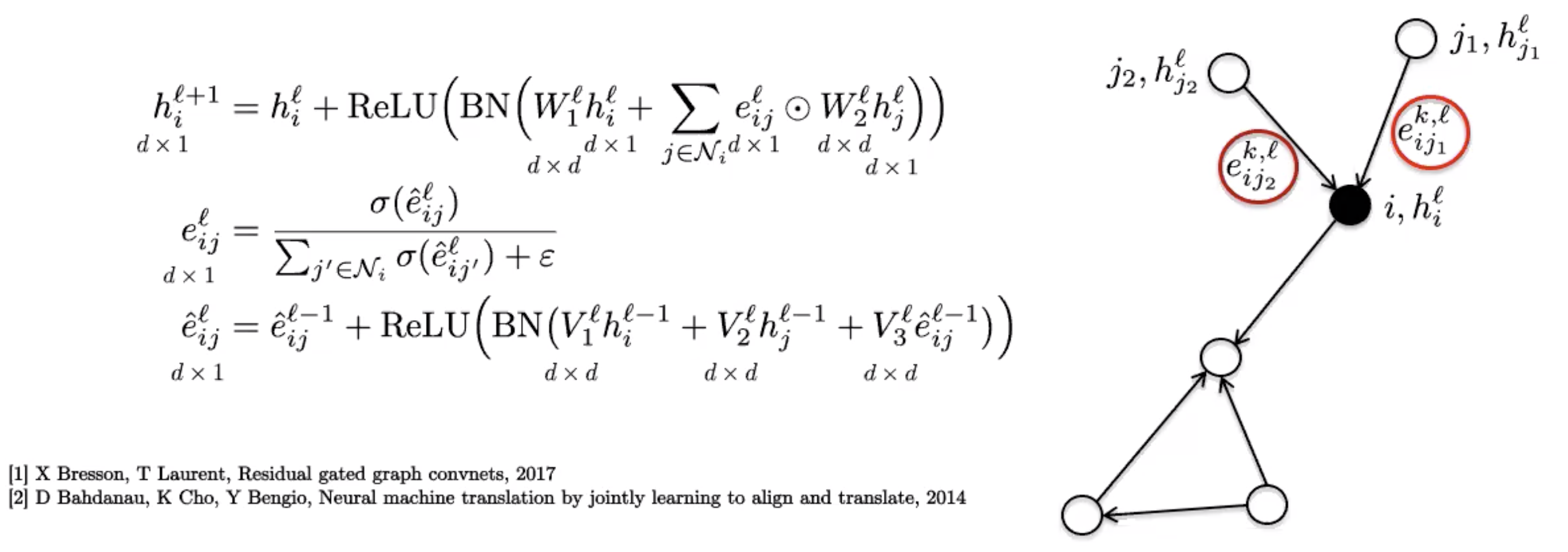
Figure 8: Gated Graph ConvNet

Graph Transformers

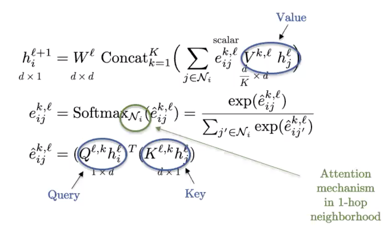
Figure 9: Graph Transformer

This is the graph version of the standard transformer, commonly used in NLP. If the graph is fully connected (every two nodes share an edge), we recover the definition of a standard transformer.

Graphs obtain their structure from sparsity, so the fully connected graph has trivial structure and is essentially a set. Transformers then can be viewed as Set Neural Networks, and are in fact the best technique currently to analyse sets/bags of features.

Benchmarking GNNs

Benchmarks are an essential part of progress in any field. The recently released benchmark Benchmarking Graph Neural Networks has six medium-scale datasets that can be used for four fundamental graph problems - graph classification, graph regression, node classification and edge classification. Though these datasets are mediumly sized, they are enough to statistically separate trends in various GNNs.

As an example of a Graph Regression task, we would want to predict the molecular solubility.

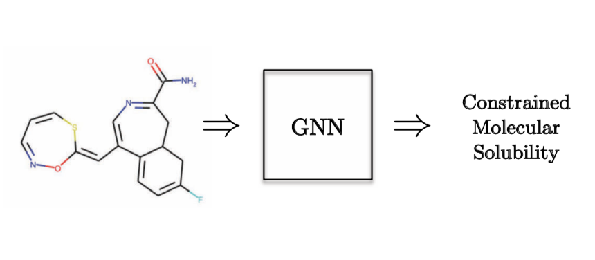
Figure 10: Graph Regression task - Quantum Chemistry

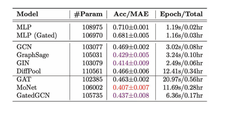
Figure 11: Performance of various GCNs on the regression task

We notice that in most cases anisotropic GCNs perform better compared to isotropic GCNs because we use directional properties.

For a Graph Classification task, a Computer Vision problem was chosen where we have super nodes of images and we want to classify the image.

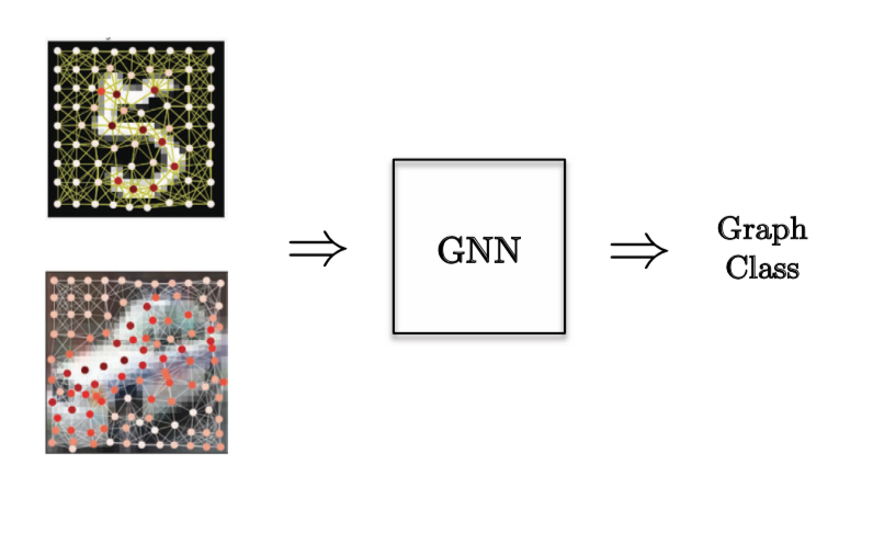
Figure 12: Graph Classification task

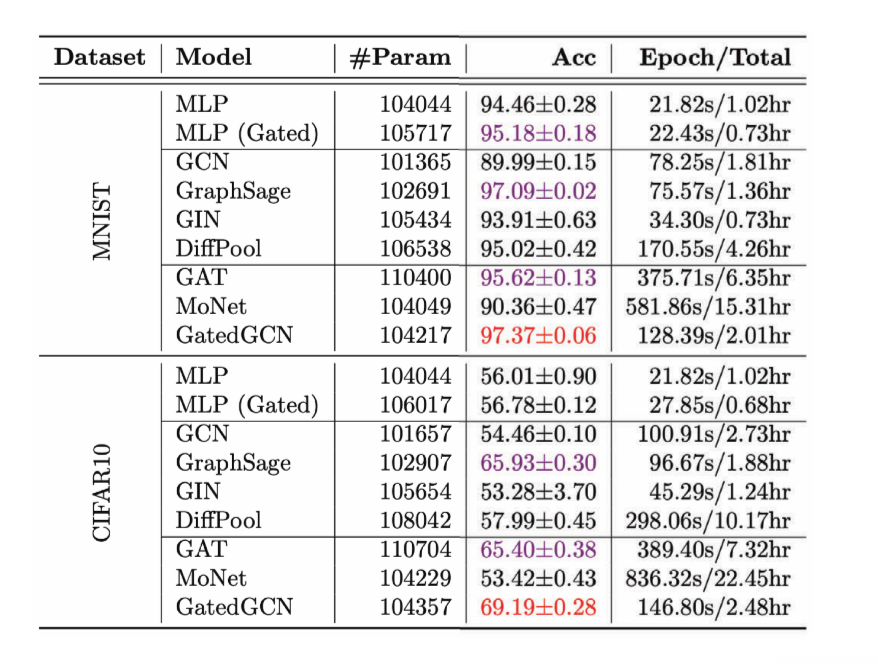
Figure 13: Performance of various GCNs on Graph Classification task

For an Edge Classification task, we have considered the Combinatorial Optimization problem of the Travelling Salesman Problem (TSP) - where we want to know if a particular edge belongs to the optimal solution. If it belongs to the solution it falls in class 1, else class 0. Here we need explicit edge features, and the only model that does a good job of this is GatedGCN.

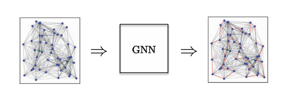
Figure 14: Edge Classification task.

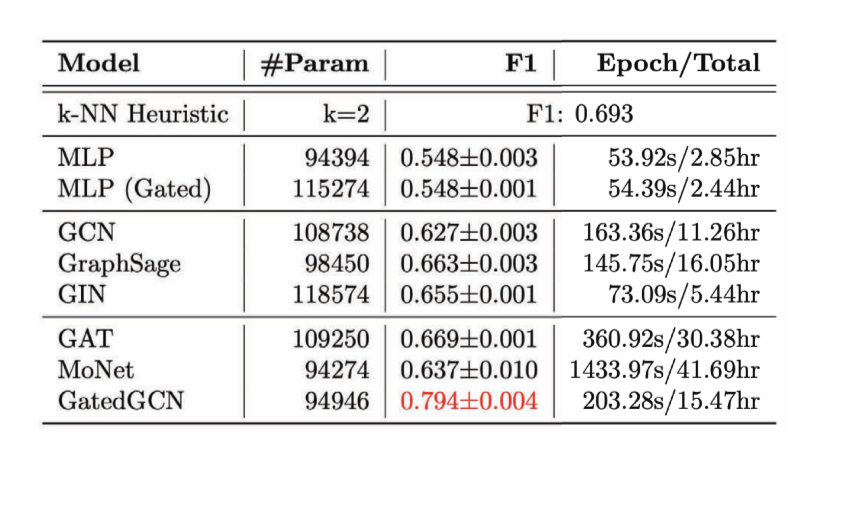
Figure 15: Performance of various GCNs on Edge Classification task

We can use GCNs for self-supervised tasks as well, they are not limited to supervised learning models. According to Dr. Yann LeCun, almost all self-supervised learning tasks exploit some sort of graph structure. When we do a self-supervised learning task in text, where we take a sequence of words and we learn to predict missing words or new sentences. There is a graphs structure here, which is how many times a word appears some distance away from another word. Text would be a linear graph, and the neighbours chosen would be used to train a Transformer. In the case of contrastive training, where we have two samples that are similar, and two which are dissimilar - it is essentially a similarity graph, where two samples are linked when they are similar and if they are not linked they are considered dissimilar.

Conclusion

GCNs generalize CNNs to data on graphs. The convolution operator needed to be redesigned on graphs. Doing this for template matching gave rise to Spatial GCNs, and for spectral convolution lead to Spectral GCNs.

There is linear complexity for sparse graphs, and GPU implementation, although the latter is not yet optimized for sparse matrix multiplication. The applications are abound as shown below.

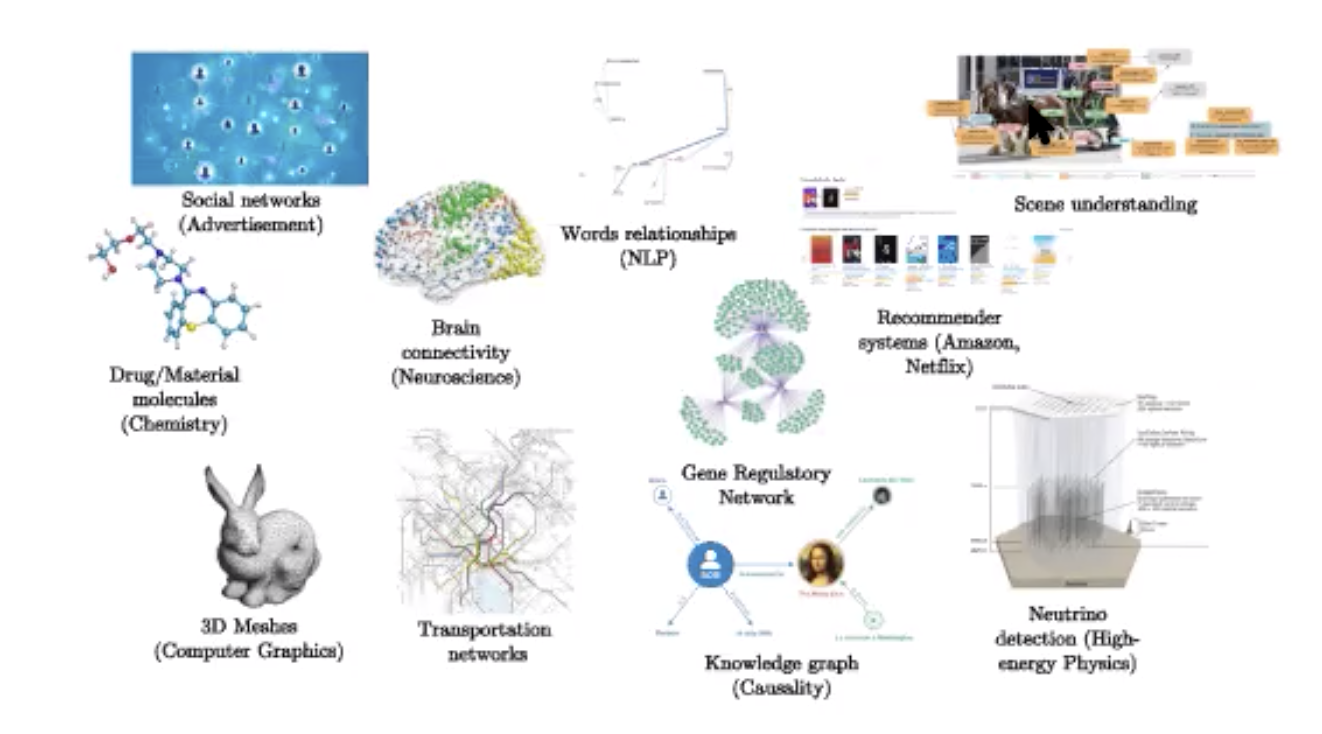
Figure 16: Applications