Overfitting and regularization

Overfitting

Consider a regression problem. A model could underfit, right-fit, or overfit.

If the model is insufficiently expressive for the data it will underfit. If the model is more expressive than the data (as is the case with deep neural networks), it runs the risk of overfitting.

In this case, the model is powerful enough to fit both the original data and the noise, producing a poor solution for the task at hand.

Ideally we would like our model to fit the underlying data and not the noise, producing a good fit for our data. We would especially like to do this without needing to reduce the power of our models. Deep learning models are very powerful, often much more than is strictly necessary in order to learn the data. We would like to keep that power (to make training easier), but still fight overfitting.

Overfitting for debugging

Overfitting can be useful in some cases, such as during debugging. One can test a network on a small subset of training data (even a single batch or a set of random noise tensors) and make sure that the network is able to overfit to this data. If it fails to learn, it is a sign that there may be a bug.

Regularization

We can try to fight overfitting by introducing regularization. The amount of regularization will affect the model’s validation performance. Too little regularization will fail to resolve the overfitting problem. Too much regularization will make the model much less effective.

Regularization adds prior knowledge to a model; a prior distribution is specified for the parameters. It acts as a restriction on the set of possible learnable functions.

Another definition of regularization from Ian Goodfellow:

Regularization is any modification we make to a learning algorithm that is intended to reduce its generalization error but not its training error.

Initialization techniques

We can select a prior for our network parameters by initializing the weights according to a particular distribution. One option: Xavier initialization.

Weight decay regularisation

Weight decay is our first regularisation technique. Weight decay is in widespread use in machine learning, but less so with neural networks. In PyTorch, weight decay is provided as a parameter to the optimizer (see for example the weight_decay parameter for SGD).

This is also called:

• L2
• Ridge
• Gaussian prior

We can consider an objective which acts on the parameters:

then we have updates:

For weight decay we add a penalty term:

which produces an update

This new term in the update drives the parameters $\theta$ slightly toward zero, adding some “decay” in the weights with each update.

L1 regularisation

Available as an option for PyTorch optimizers.

Also called:

• LASSO: Least Absolute Shrinkage Selector Operator
• Laplacian prior
• Sparsity prior

Viewing this as a Laplace distribution prior, this regularization puts more probability mass near zero than does a Gaussian distribution.

Starting with the same update as above we can view this as adding another penalty:

which produces an update

Unlike $L_2$ weight decay, the $L_1$ regularization will “kill” components that are close to an axis in the parameter space, rather than evenly reducing the length of the parameter vector.

Dropout

Dropout involves setting a certain number of neurons to zero randomly during training. This prevents the network from learning a singular path from input to output. Similarly, due to the large parametrisation of neural networks, it is possible for the neural network to effectively memorize the input. However, with dropout, this is a lot more difficult since the input is being put into a different network each time since dropout effectively trains a infinite number of networks that are different each time. Hence, dropout can be a powerful way of controlling overfitting and being more robust against small variations in the input.

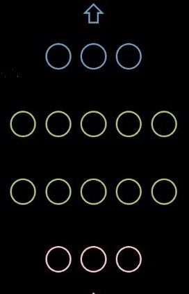
Figure 1: Network without dropout

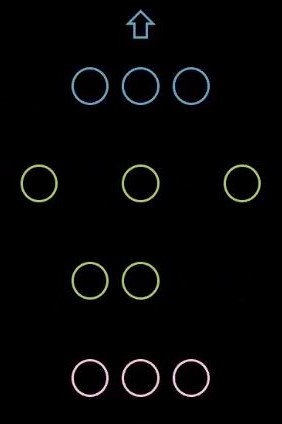
Figure 2: Network with dropout

In PyTorch, we can set a random dropout rate of neuron.

Figure 3: Dropout code

After training, during inference, dropout is not used any more. In order to create the final network for inference, we average over all of the individual networks created during dropout and use that for inference. We can similarly multiply all of the weights by $1/1-p$ where $p$ is the dropout rate.

Early-stopping

During training, if the validation loss starts increasing, we can stop training and use the best weights found so far. This prevents the weights from growing too much which will start hurting validation performance at some point. In practise, it is common to calculate the validation performance at certain intervals and stop after a certain number of validation error calculations stop decreasing.

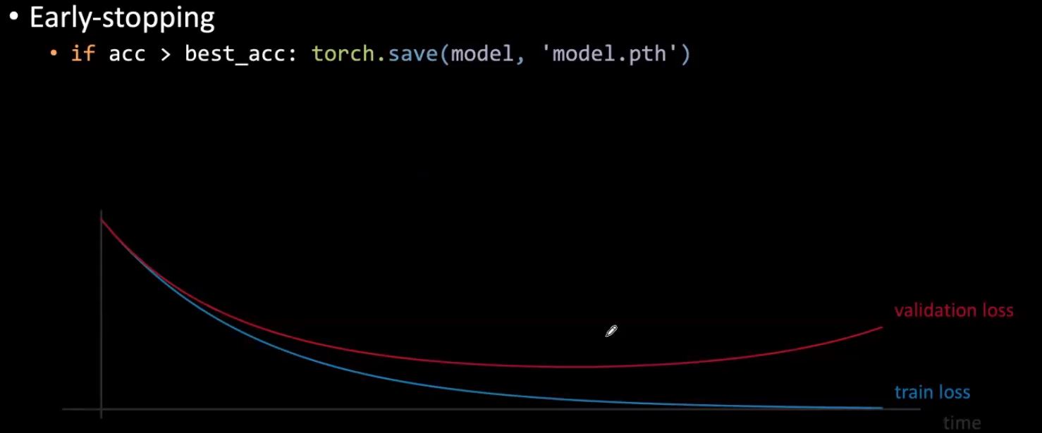
Figure 4: Early stopping

Fighting overfitting indirectly

There are techniques that have the side-effect of regularizing parameters but are not regularisers themselves.

Batch-norm

Q. How does batch norm make training more efficient? A. We can use higher learning rate when applying batch norm.

Batch normalization is used to prevent the internal covariate shift of a neural network but there is a lot debate if it actually does this and what the true benefit actually is.

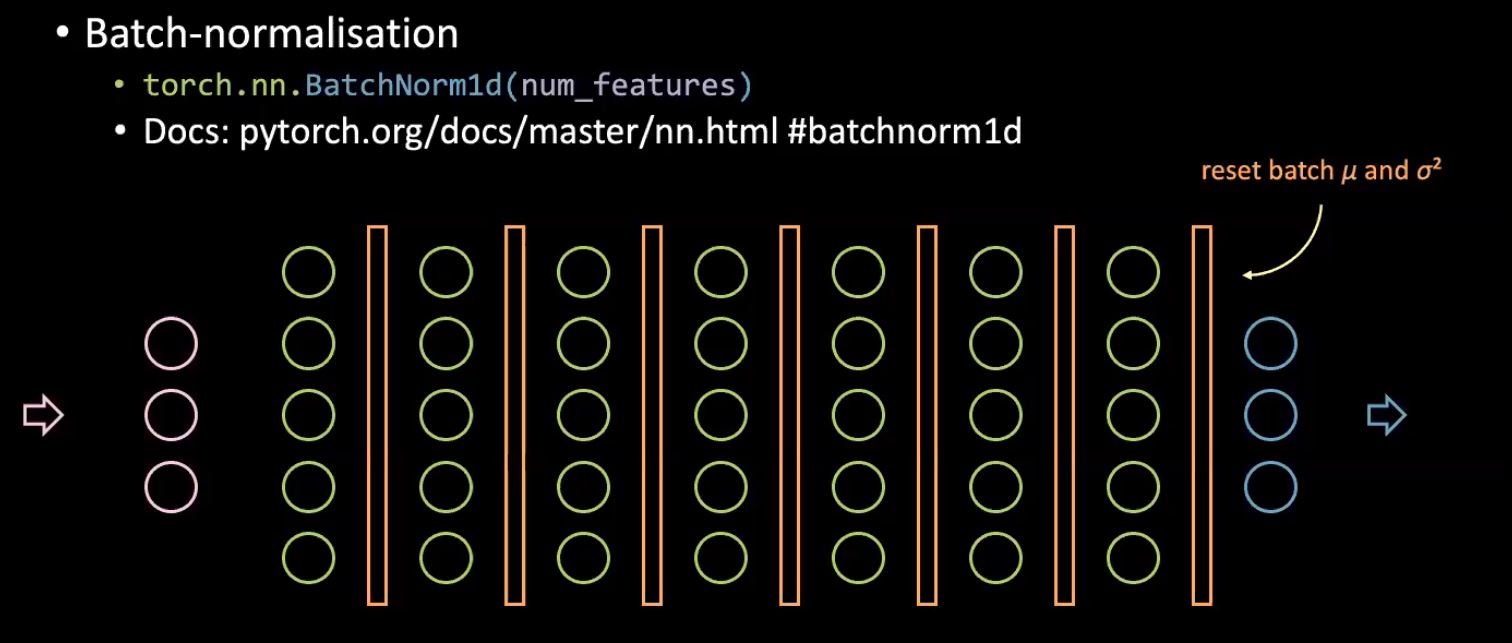
Figure 5: Batch normalization

Batch normalisation essentially extends the logic of normalizing the input of the neural network to normalizing the input of each hidden layer in the network. The basic idea is to have a fixed distribution feed each subsequent layer of a neural network since learning occurs best when we have a fixed distribution. To do this, we compute the mean and variance of each batch before each hidden layer and normalize the incoming values by these batch specific statistics, which reduces the amount by which the values will ultimately shift around during training.

Regarding the regularizing effect, due to each batch being different, each sample will be normalized by slightly different statistics based upon the batch it is in. Hence, the network will see various slightly altered versions of a single input which helps the network learn to be more robust against slight variations in the input and prevent overfitting.

Another benefit of batch normalisation is that training is a lot faster.

More data

Gathering more data is a easy way to prevent overfitting but can be expensive or not feasible.

Data-augmentation

Transformations using Torchvision can have a regularizing effect by teaching the network to learn how to be insensitive to perturbations.

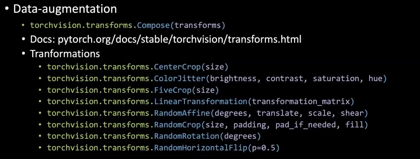
Figure 6: Data augmentation with Torchvision.

Transfer leaning (TF) fine-tuning (FT)

Transfer learning (TF) refers to just training a final classifier on top of a pre-trained network (used in cases of little data generally).

Fine tuning (FT) refers to training partial/full portions of the pre-trained network as well (used in cases where we have a lot of data generally).

Q. Generally, when should we freeze the layers of a pre-trained model? A. If we have little training data.

4 general cases: 1) If we have little data with similar distributions, we can just do transfer learning. 2) If we have a lot of data with similar distributions we can do fine-tuning in order to improve the performance of the feature extractor as well. 3) If we have a little data and a different distribution we should remove a few of the final trained layers in the feature extractor since they are too specialized. 4) If we have a lot of data and they are from different distributions, we can just train all portions.

Note, we can also use different learning rates for different layers in order to improve performance.

To further our discussion about overfitting and regularisation, let us look at the visualisations below. These visualisations were generated with the code from Notebook.

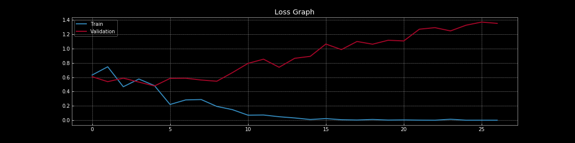
Figure 7: Loss curves without dropout

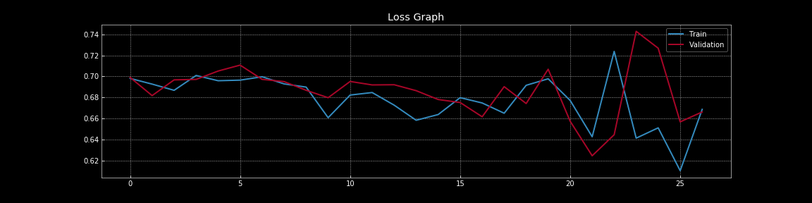
Figure 8: Loss curves with dropout

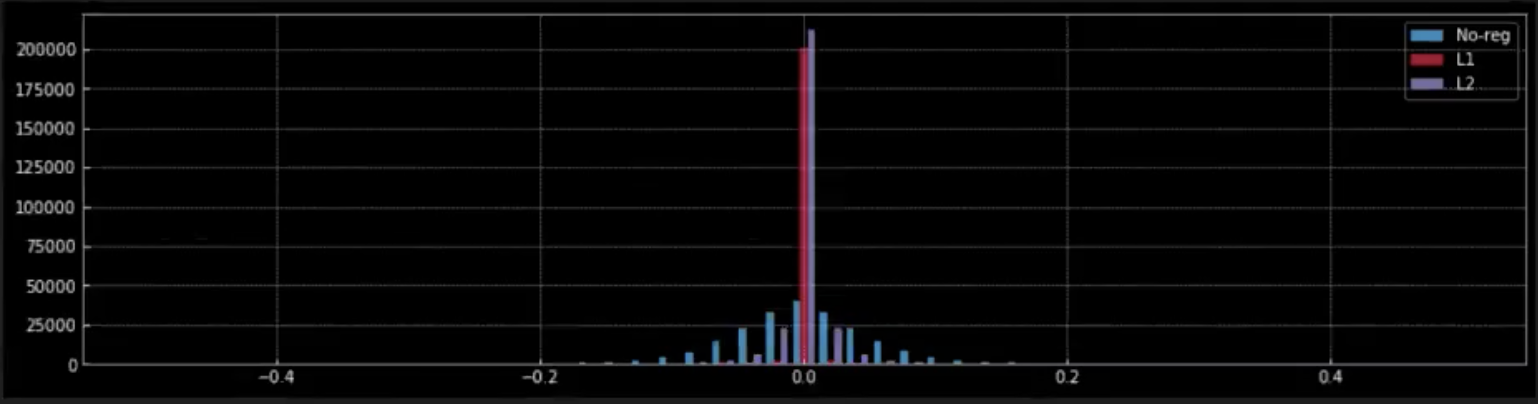
Figure 9: Effect of regularization on weights

From Figure 7 and Figure 8, we can understand the dramatic effect that dropout has on generalisation error i.e. the difference between the training loss and validation loss. In Figure 7, without dropout there is clear overfitting as the training loss is much lower than the validation loss. However, in Figure 8, with dropout the training loss and validation loss almost continuously overlap indicating that the model is generalising well to the validation set, which serves as our proxy for out-of-sample set. Of course, we can measure the actual out-of-sample performance using a separate holdout test set.

In Figure 9, we observe the effect that regularisation (L1 & L2) have on the weights of the network.

• When we apply L1 regularisation, from the red peak at zero, we can understand that most of the weights are zero. Small red dots closer to zero are the non-zero weights of the model.

• Contrastingly, in L2 regularisation, from the lavender peak near zero we can see that most of the weights are close to zero but non-zero.

• When there is no regularisation (blue) the weights are much more flexible and spread out around zero resembling a normal distribution.

Bayesian Neural Networks: estimating uncertainty around predictions

We care about uncertainty in neural networks because a network needs to know how certain/confident on its prediction.

Ex: If you build a neural networks to predict steering control, you need to know how confident the network’s predictions.

We can use a neural network with dropout to get a confidence interval around our predictions. Let us train a network with dropout, $r$ being the dropout ratio.

Usually during inference, we set the network to validation mode and use all neurons to get the final prediction. While doing the prediction, we scale the weights $\delta$ by $\dfrac{1}{1-r}$ to account for dropping neurons during training.

This method gives us a single prediction for each input. However, to get a confidence interval around our prediction, we need multiple predictions for the same input. So instead of setting the network to validation mode during inference, we retain it in training mode i.e. still drop neurons randomly and get a prediction. When we predict multiple times using this dropout network, for the same input we will get different predictions depending on the neurons being dropped. We use these predictions to estimate the average final prediction and a confidence interval around it.

In the below images, we have estimated confidence intervals around the predictions of networks. These visualisations were generated with the code from Bayesian Neural Networks Notebook. The red line represents the predictions. The purple shaded region around the predictions represent the uncertainty i.e. variance of predictions.

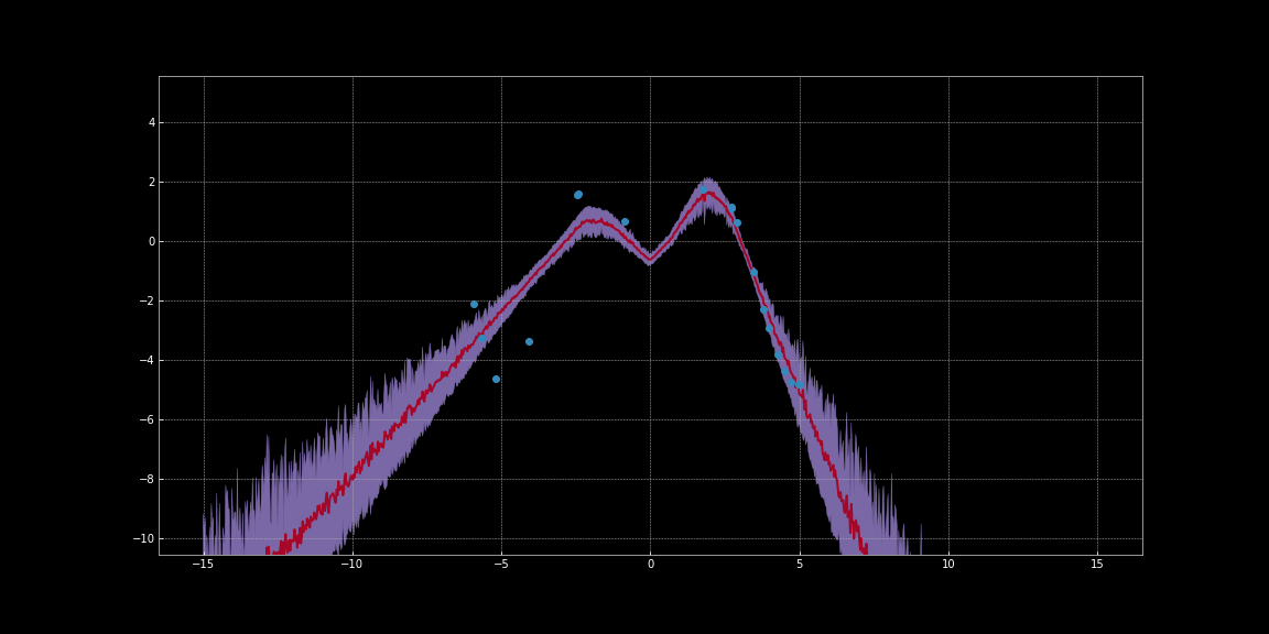
Figure 10: Uncertainty Estimation using ReLU activation

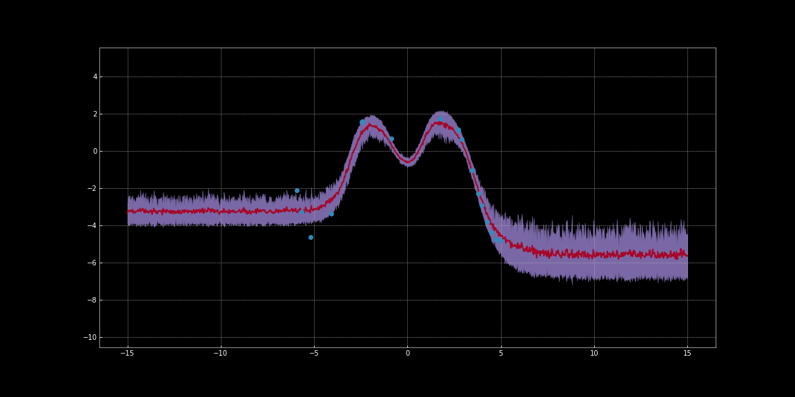
Figure 11: Uncertainty Estimation using Tanh activation

As you can observe in the above images, these uncertainty estimations are not calibrated. They are different for different activation functions. Noticeably in the images, uncertainty around data points is low. Furthermore, the variance that we can observe is a differentiable function. So we can run gradient descent to minimise this variance. Thereby we can get more confident predictions.

If we have multiple terms contributing to total loss in our EBM model, how do they interact?

In EBM models, we can simply and conveniently sum the different terms to estimate the total loss.

Digression: A term that penalises the length of the latent variable can act as one of many loss terms in a model. The length of a vector is roughly proportional to the number of dimensions it has. So if you decrease the number of dimensions, then the length of the vector decreases and as a result it encodes less information. In an auto-encoder setting, this makes sure that the model is retaining the most important information. So, one way to bottleneck information in latent spaces is to reduce the dimensionality of the latent space.

How can we determine the hyper-parameter for regularisation?

In practice, to determine the optimal hyper-parameter for regularisation i.e. regularisation strength we can use

• Bayesian hyper-parameter Optimization
• Grid Search
• Random Search

While doing these searches, the first few epochs are usually enough to give us a sense of how the regularization is working. So we need train the model extensively.