Deep Learning for NLP

Overview

• Amazing progress in recent years:
  • Humans prefer machine translation to human translators for some languages
  • Super-human performance on many question answering datasets
  • Language models generate fluent paragraphs (e.g Radford et al. 2019)
• Minimal specialist techniques needed per task, can achieve these things with fairly generic models

Language Models

• Language models assign a probability to a text: $p(x_0, \cdots, x_n)$
• Many possible sentences so we can’t just train a classifier
• Most popular method is to factorize distribution using chain rule:

Neural Language Models

Basically we input the text into a neural network, the neural network will map all this context onto a vector. This vector represents the next word and we have some big word embedding matrix. The word embedding matrix contains a vector for every possible word the model can output. We then compute similarity by dot product of the context vector and each of the word vectors. We’ll get a likelihood of predicting the next word, then train this model by maximum likelihood. The key detail here is that we don’t deal with words directly, but we deal with things called sub-words or characters.

Fig.1: Neural language model

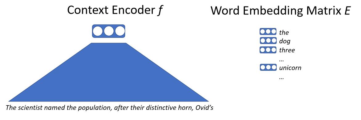
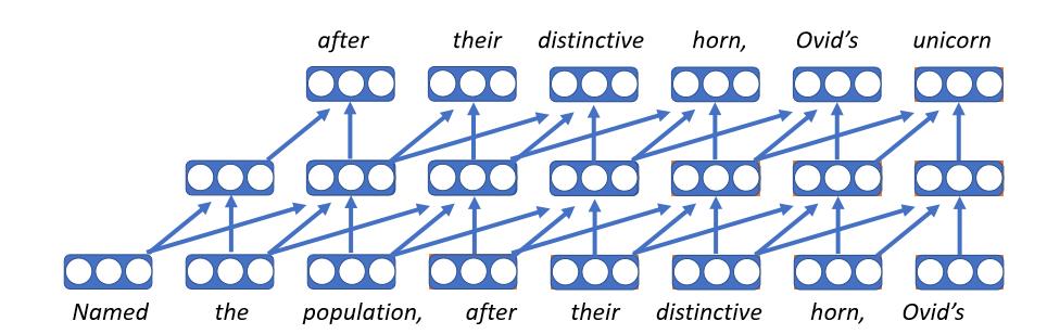
Convolutional Language Models

• The first neural language model
• Embed each word as a vector, which is a lookup table to the embedding matrix, so the word will get the same vector no matter what context it appears in
• Apply same feed forward network at each time step
• Unfortunately, fixed length history means it can only condition on bounded context
• These models do have the upside of being very fast

Fig.2: Convolutional language model

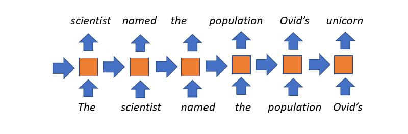
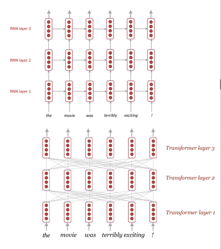
Recurrent Language Models

• The most popular approach until a couple years ago.
• Conceptually straightforward: every time step we maintain some state (received from the previous time step), which represents what we’ve read so far. This is combined with current word being read and used at later state. Then we repeat this process for as many time steps as we need.
• Uses unbounded context: in principle the title of a book would affect the hidden states of last word of the book.
• Disadvantages:
  • The whole history of the document reading is compressed into fixed-size vector at each time step, which is the bottleneck of this model
  • Gradients tend to vanish with long contexts
  • Not possible to parallelize over time-steps, so slow training

Fig.3: Recurrent language model

Transformer Language Models

• Most recent model used in NLP
• Revolutionized penalty
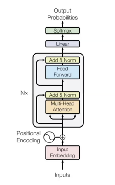
• Three main stages
  • Input stage
  • $n$ times transformer blocks (encoding layers) with different parameters
  • Output stage
• Example with 6 transformer modules (encoding layers) in the original transformer paper:

Fig.4:Transformer language model

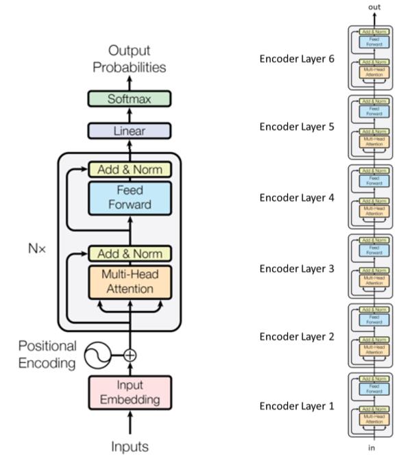
Sub-layers are connected by the boxes labelled “Add&Norm”. The “Add” part means it is a residual connection, which helps in stopping the gradient from vanishing. The norm here denotes layer normalization.

Fig.5: Encoder Layer

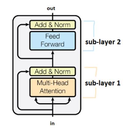
It should be noted that transformers share weights across time-steps.

Multi-headed attention

Fig.6: Multi-headed Attention

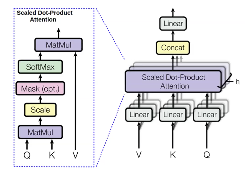
For the words we are trying to predict, we compute values called query(q). For all the previous words use to predict we call them keys(k). Query is something that tells about the context, such as previous adjectives. Key is like a label containing information about the current word such as whether it’s an adjective or not. Once q is computed, we can derive the distribution of previous words ($p_i$):

Then we also compute quantities called values(v) for the previous words. Values represent the content of the words.

Once we have the values, we compute the hidden states by maximizing the attention distribution:

We compute the same thing with different queries, values, and keys multiple times in parallel. The reason for this is that we want to predict the next word using different things. For example, when we predict the word “unicorns” using three previous words “These” “horned” and “silver-white”. We know it is a unicorn by “horned” “silver-white”. However, we can know it is plural “unicorns” by “These”. Therefore, we probably want to use all these three words to know what the next word should be. Multi-headed attention is a way of letting each word look at multiple previous words.

One big advantage about the multi-headed attention is that it is very parallelisable. Unlike RNNs, it computes all heads of the multi-head attention modules and all the time-steps at once. One problem of computing all time-steps at once is that it could look at futures words too, while we only want to condition on previous words. One solution to that is what is called self-attention masking. The mask is an upper triangular matrix that have zeros in the lower triangle and negative infinity in the upper triangle. The effect of adding this mask to the output of the attention module is that every word to the left has a much higher attention score than words to the right, so the model in practice only focuses on previous words. The application of the mask is crucial in language model because it makes it mathematically correct, however, in text encoders, bidirectional context can be helpful.

One detail to make the transformer language model work is to add the positional embedding to the input. In language, some properties like the order are important to interpret. The technique used here is learning separate embeddings at different time-steps and adding these to the input, so the input now is the summation of word vector and the positional vector. This gives the order information.

Fig.7: Transformer Architecture

Why the model is so good:

1. It gives direct connections between each pair of words. Each word can directly access the hidden states of the previous words, mitigating vanishing gradients. It learns very expensive function very easily
2. All time-steps are computed in parallel
3. Self-attention is quadratic (all time-steps can attend to all others), limiting maximum sequence length

Some tricks (especially for multi-head attention and positional encoding) and decoding Language Models

Trick 1: Extensive use of layer normalization to stabilize training is really helpful

• Really important for transformers

Trick 2: Warm-up + Inverse-square root training schedule

• Make use of learning rate schedule: in order to make the transformers work well, you have to make your learning rate decay linearly from zero to thousandth steps.

Trick 3: Careful initialization

• Really helpful for a task like machine translation

Trick 4: Label smoothing

• Really helpful for a task like machine translation

The following are the results from some methods mentioned above. In these tests, the metric on the right called ppl was perplexity (the lower the ppl the better).

Fig.8: Model Performance Comparison

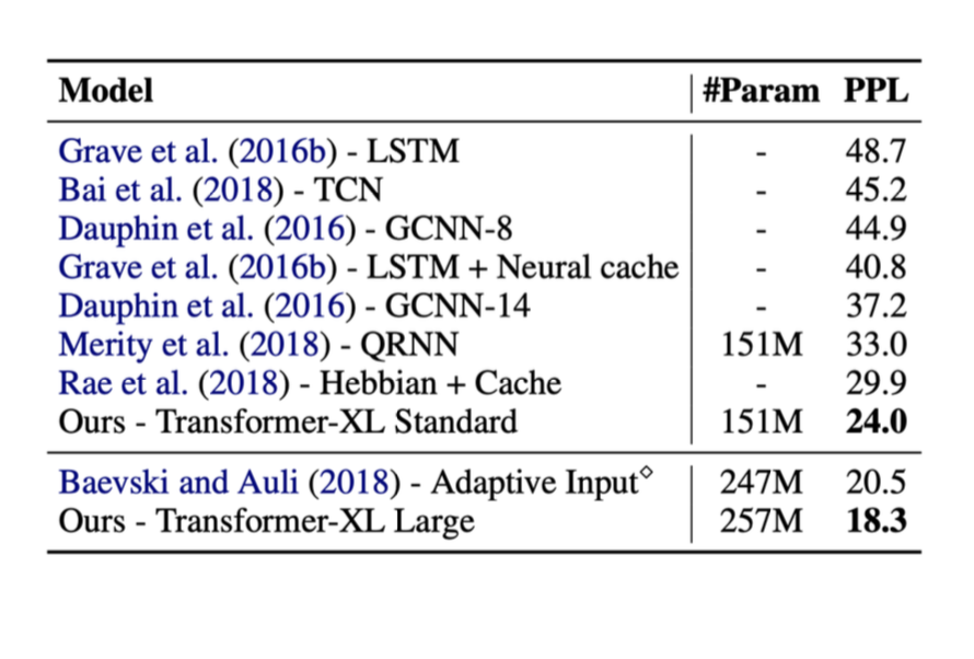
You could see that when transformers were introduced, the performance was greatly improved.

Some important facts of Transformer Language Models

• Minimal inductive bias
• All words directly connected, which will mitigate vanishing gradients.

• All time-steps computed in parallel.

• Self attention is quadratic (all time-steps can attend to all others), limiting maximum sequence length.

• As self attention is quadratic, its expense grows linearly in practice, which could cause a problem.

Fig.9: Transformers *vs.* RNNs

Transformers scale up very well

1. Unlimited training data, even far more than you need
2. GPT 2 used 2 billion parameters in 2019
3. Recent models use up to 17B parameters in 2020

Decoding Language Models

We can now train a probability distribution over text - now essentially we could get exponentially many possible outputs, so we can’t compute the maximum. Whatever choice you make for your first word could affect all the other decisions. Thus, given that, the greedy decoding was introduced as follows.

Greedy Decoding does not work

We take most likely word at each time step. However, no guarantee this gives most likely sequence because if you have to make that step at some point, then you get no way of back-tracking your search to undo any previous sessions.

Exhaustive search also not possible

It requires computing all possible sequences and because of the complexity of $O(V^T)$, it will be too expensive

Comprehension Questions and Answers

1. What is the benefit of multi-headed attention as opposed to a single-headed attention model?

   • To predict the next word you need to observe multiple separate things, in other words attention can be placed on multiple previous words in trying to understand the context necessary to predict the next word.

2. How do transformers solve the informational bottlenecks of CNNs and RNNs?

   • Attention models allow for direct connection between all words allowing for each word to be conditioned on all previous words, effectively removing this bottleneck.

3. How do transformers differ from RNNs in the way they exploit GPU parallelization?

   • The multi-headed attention modules in transformers are highly parallelisable whereas RNNs are not and therefore cannot take advantage of GPU technology. In fact transformers compute all time steps at once in single forward pass.