Prediction and Policy learning Under Uncertainty (PPUU)

Introduction and problem setup

Let us say we want to learn how to drive in a model-free Reinforcement learning way. We train models in RL by letting the model make mistakes and learn from them. But this is not the best way since mistakes might take us to heaven/hell where there is no point in learning.

So, let us talk about a more ‘human’ way to learn how to drive a car. Consider an example of lane switching. Assuming the car is moving at 100 km/h, which roughly translates to 30 m/s, if we look 30 m in front of us, we are roughly looking 1 s into the future.

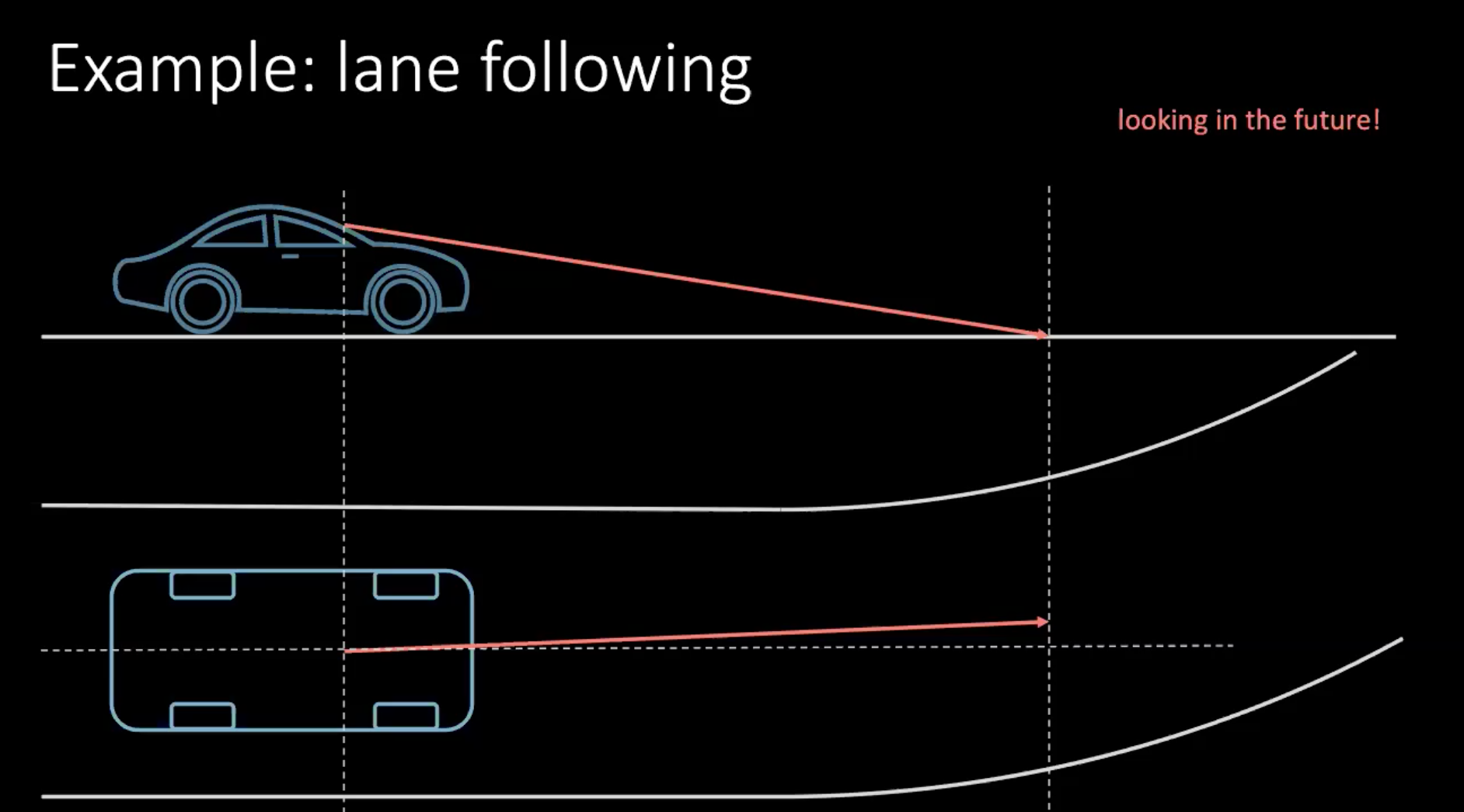
Figure 1: Looking into future while driving

If we were turning, we need to make a decision based on the near future. To take a turn in a few meters, we take an action now, which in this context is turning the steering wheel. Making a decision not only depends on your driving but also the surrounding vehicles in the traffic. Since everyone around us is not so deterministic, it is very hard to take every possibility into account.

Let us now break down what is happening in this scenario. We have an agent(represented here by a brain) that takes the input $s_t$ (position, velocity and context images) and produces an action $a_t$(steering control, acceleration and braking). The environment takes us to a new state and returns a cost $c_t$.

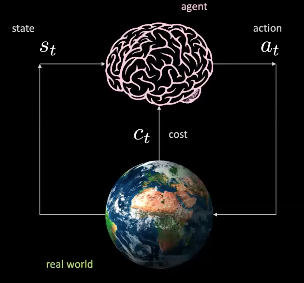
Figure 2: Illustration of an agent in the real world

This is like a simple network where you take actions given a specific state and the world gives us the next state and the next consequence. This is model-free because with every action we are interacting with the real world. But can we train an agent without actually interacting with the real world?

Yes, we can! Let us find out in the “Learning world model” section.

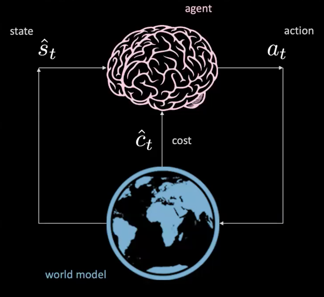
Figure 3: Illustration of an agent in the world model

Data set

Before discussing how to learn the world model, let us explore the dataset we have. We have 7 cameras mounted on top of a 30 story building facing the interstate. We adjust the cameras to get the top-down view and then extract bounding boxes for each vehicle. At a time $t$, we can determine $p_t$ representing the position, $v_t$ representing the velocity and $i_t$ representing the current traffic state around the vehicle.

Since we know the kinematics of the driving, we can invert them to figure out what are the actions that the driver is taking. For example, if the car is moving in a rectilinear uniform motion, we know that the acceleration is zero(meaning there is no action)

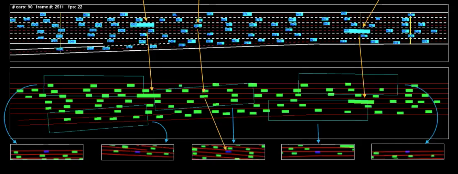
Figure 4: Machine representation of a single frame

The illustration in blue is the feed and the illustration in green is what we can call the machine representation. To understand this better, we have isolated a few vehicles(marked in the illustration). The views we see below are the bounding boxes of the field-of-view of these vehicles.

Cost

There are two different types of costs here: lane cost and proximity cost. Lane cost tells us how well we are within a lane and proximity cost tells us how close we are to the other cars.

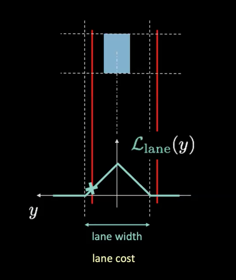
Figure 5: Lane cost

In the above figure, dotted lines represent actual lanes and red lines help us figure out the lane cost given the current position of our car. Red lines move as our car moves. The height of the intersection of the red lines with the potential curve (in cyan) gives us the cost. If the car is in the centre of the lane, both the red lines overlap with the actual lanes resulting in zero cost. On the other hand, as the car moves away from the centre, the red lines also move to result in a non-zero cost.

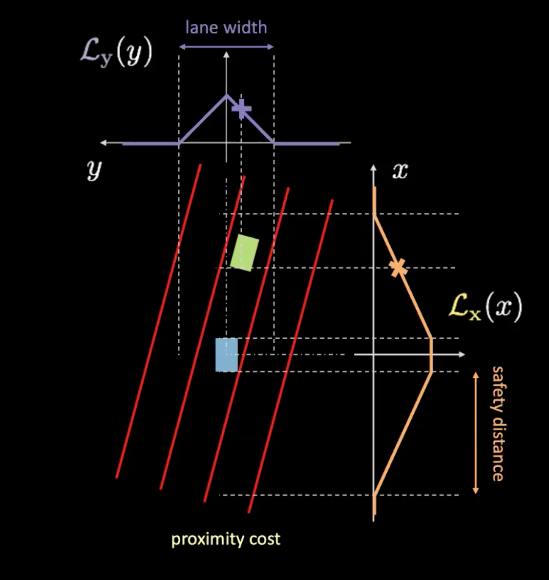
Figure 6: Proximity cost

Proximity cost has two components ($\mathcal{L}_x$ and $\mathcal{L}_y$). $\mathcal{L}_y$ is similar to the lane cost and $\mathcal{L}_x$ depends on the speed of our car. The Orange curve in Figure 6 tells us about the safety distance. As the speed of the car increases, the orange curve widens. So faster the car is travelling, the more you will need to look ahead and behind. The height of the intersection of a car with the orange curve determines $\mathcal{L}_x$.

The product of these two components gives us the proximity cost.

Learning world model

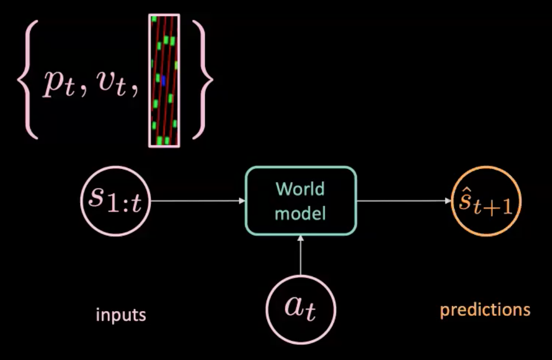
Figure 7: Illustration of the world model

The world model is fed with an action $a_t$ (steering, brake, and acceleration) and $s_{1:t}$ (sequence of states where each state is represented by position, velocity and context images at that time) and it predicts the next state $\hat s_{t+1}$. On the other hand, we have the real world which tells us what actually happened ($s_{t+1}$). We optimize MSE (Mean Squared Error) between prediction ($\hat s_{t+1}$) and target ($s_{t+1}$) to train our model.

Deterministic predictor-decoder

One way to train our world model is by using a predictor-decoder model explained below.

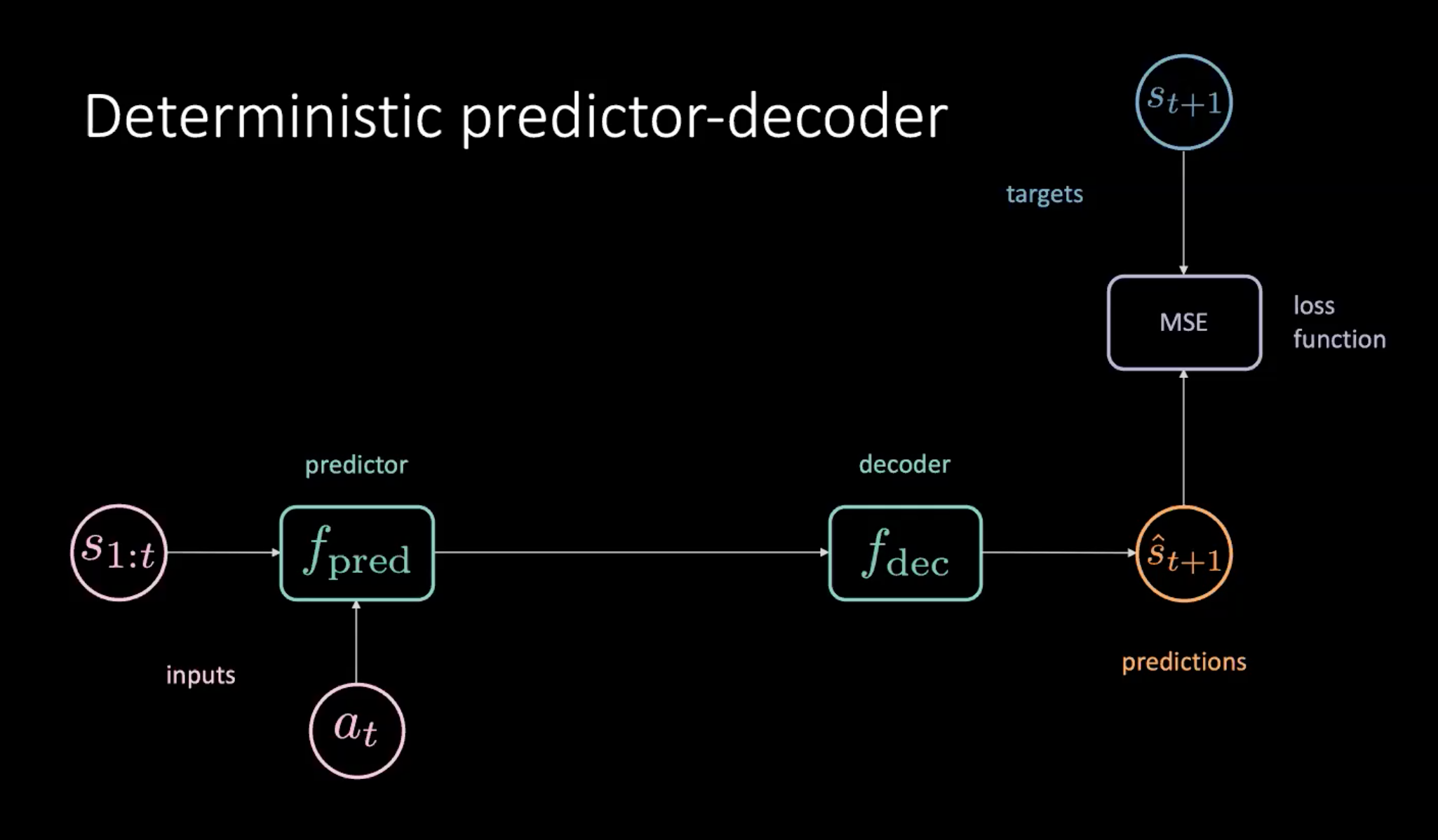
Figure 8: Deterministic predictor-decoder to learn the world model

As depicted in Figure 8, we have a sequence of states($s_{1:t}$) and action ($a_t$) which are provided to the predictor module. The predictor outputs a hidden representation of the future which is passed on to the decoder. The decoder is decoding the hidden representation of the future and outputs a prediction($\hat s_{t+1}$). We then train our model by minimising MSE between prediction $\hat s_{t+1}$ and target $s_{t+1}$.

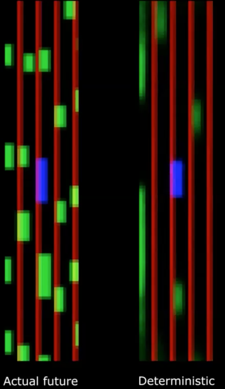
Figure 9: Actual future *vs.* Deterministic future

Unfortunately, this does not work!

We see that the deterministic output becomes very hazy. This is because our model is averaging over all the future possibilities. This can be compared to the future’s multimodality discussed a couple of classes earlier, where a pen placed at origin is dropped randomly. If we take the average across all locations, it gives us a belief that pen never moved which is incorrect.

We can address this problem by introducing latent variables in our model.

Variational predictive network

To solve the problem stated in the previous section, we add a low dimensional latent variable $z_t$ to the original network which goes through an expansion module $f_{exp}$ to match the dimensionality.

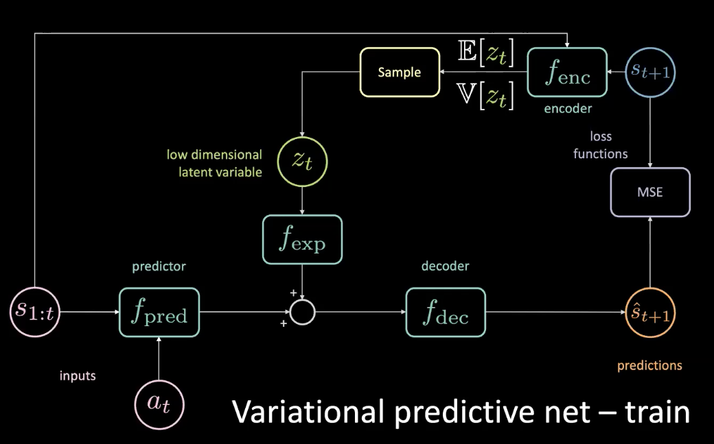
Figure 10: Variational predictive network - train

The $z_t$ is chosen such that the MSE is minimized for a specific prediction. By tuning the latent variable, you can still get MSE to zero by doing gradient descent into latent space. But this is very expensive. So, we can actually predict that latent variable using an encoder. Encoder takes the future state to give us a distribution with a mean and variance from which we can sample $z_t$.

During training, we can find out what is happening by looking into the future and getting information from it and use that information to predict the latent variable. However, we don’t have access to the future during testing time. We fix this by enforcing the encoder to give us a posterior distribution as close as possible to the prior by optimizing KL divergence.

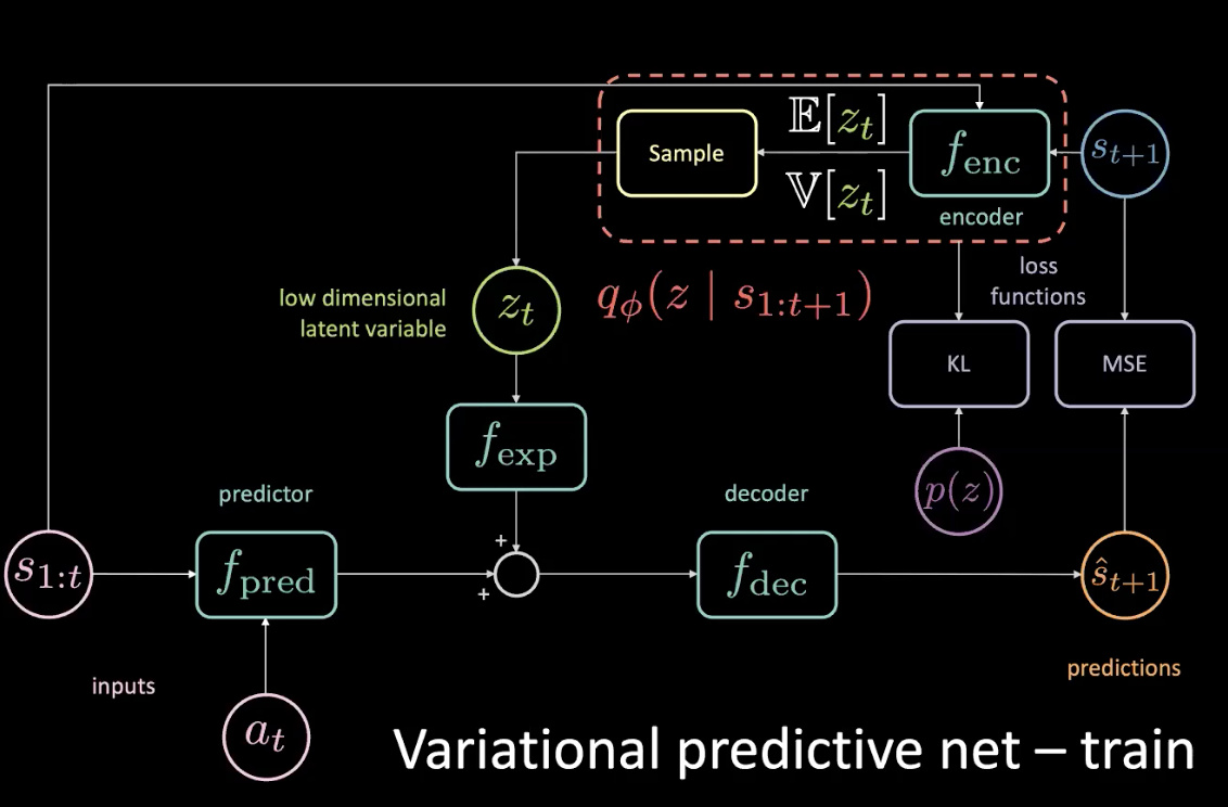
Figure 11: Variational predictive network - train (with prior distribution)

Now, let us look at the inference - How do we drive?

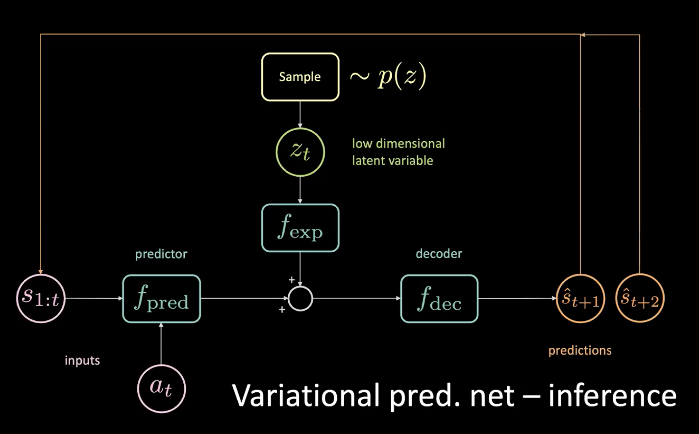
Figure 12: Variational predictive network - inference

We sample the low-dimensional latent variable $z_t$ from the prior by enforcing the encoder to shoot it towards this distribution. After getting the prediction $\hat s_{t+1}$, we put it back (in an auto-regressive step) and get the next prediction $\hat s_{t+2}$ and keep feeding the network this way.

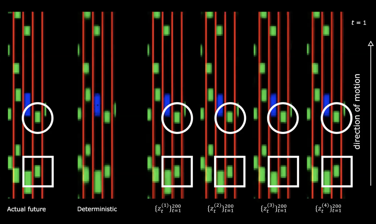
Figure 13: Actual future *vs.* Deterministic

On the right hand side in the above figure, we can see four different draws from the normal distribution. We start with same initial state and provide different 200 values to the latent variable.

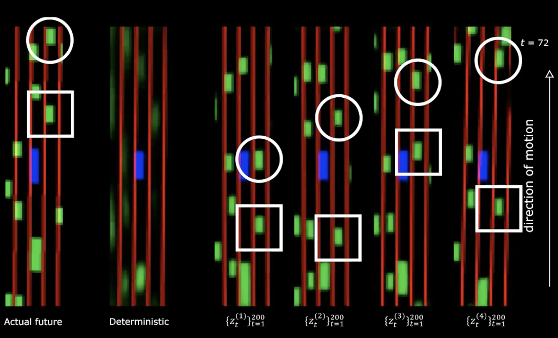
Figure 14: Actual future *vs.* Deterministic - after movement

We can notice that providing different latent variables generates different sequences of states with different behaviours. Which means we have a network that generates the future. Quite fascinating!

What’s next?

We can now use this huge amount of data to train our policy by optimizing the lane and proximity costs described above.

These multiple futures come from the sequence of latent variables that you feed to the network. If you perform gradient ascent - in the latent space, you try to increase the proximity cost so you get the sequence of latent variables such that the other cars are going to be driving into you.

Action insensitivity & latent dropout

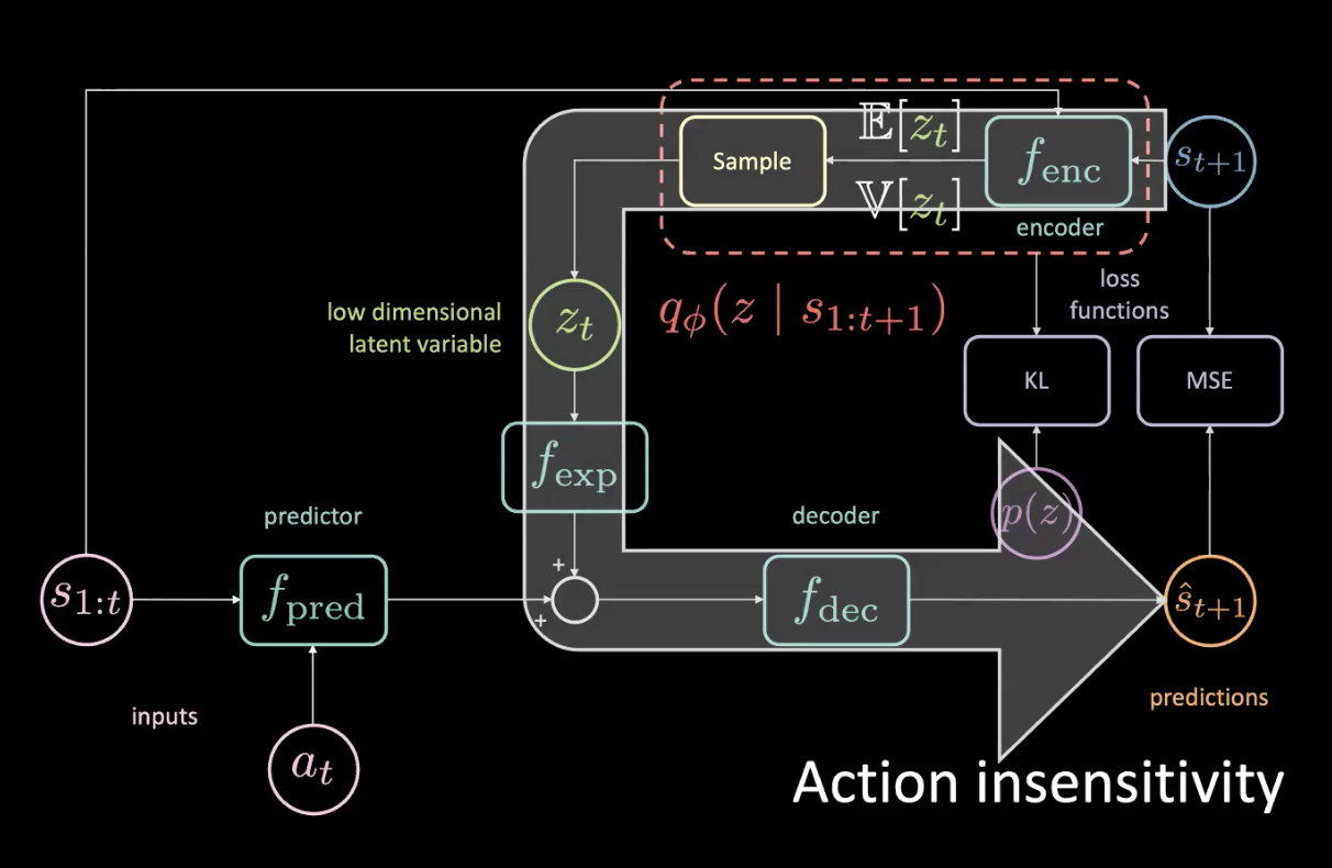
Figure 15: Issues - Action Insensitivity

Given that you actually have access to the future, if you turn to the left even slightly, everything is going to be turning to the right and that will contribute in a huge way to the MSE. The MSE loss can be minimized if the latent variable can inform the bottom part of the network that everything is going to turn to the right - which is not what we want! We can tell when everything turns to the right since that is a deterministic task.

The big arrow in Figure 15 signifies a leak of information and therefore it was not any more sensitive to the current action being provided to the predictor.

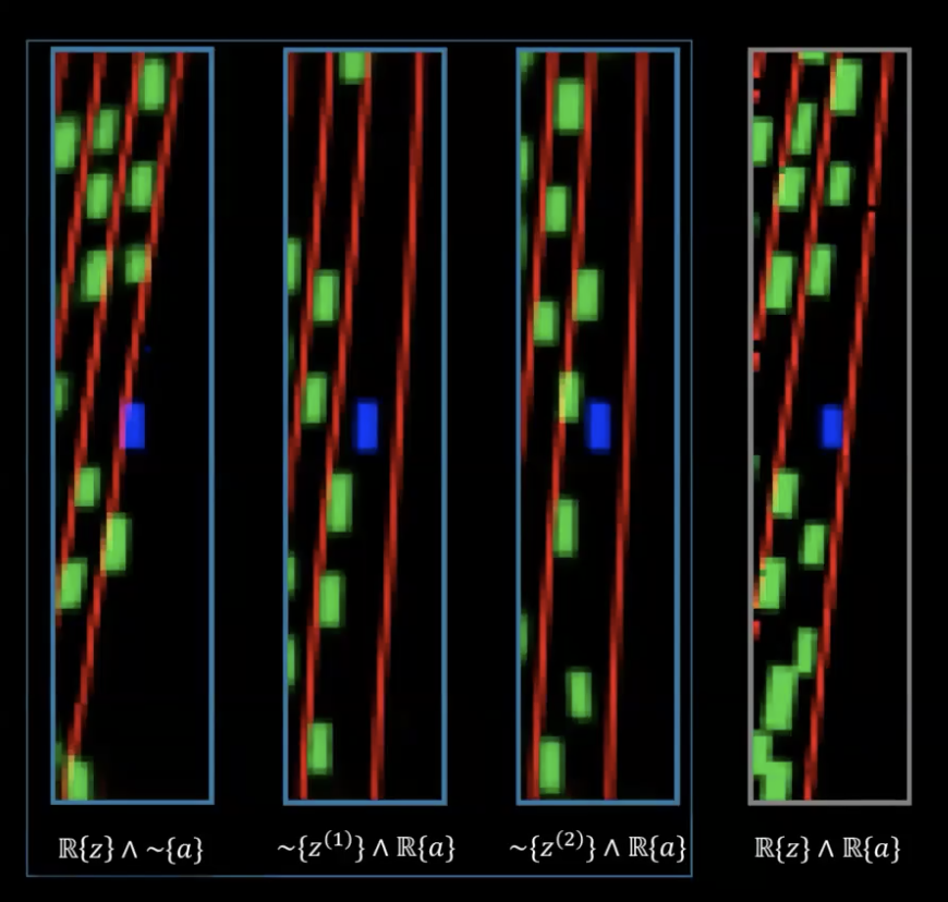
Figure 16: Issue - Action Insensitivity

In figure 16, in the rightmost diagram we have the real sequence of latent variables (the latent variables that allow us to get the most precise future) and we have the real sequence of actions taken by the expert. The two figures to the left of this one have randomly sampled latent variables but the real sequence of actions so we expect to see the steering. The last one on the left-hand side has the real sequence of latent variable but arbitrary actions and we can clearly see that the turning came mostly from the latent rather than the action, which encodes the rotation and the action (which are sampled from other episodes).

How to fix this problem?

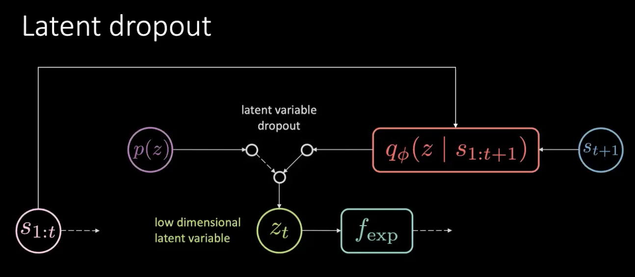
Figure 17: Fix - Latent Dropout

The problem is not a memory leak but an information leak. We fix this problem by simply dropping out this latent and sampling it from the prior distribution at random. We don’t always rely on the output of the encoder ($f_{enc}$) but pick from the prior. In this way, you cannot encode the rotation in the latent variable any more. In this way, information gets encoded in the action rather than the latent variable.

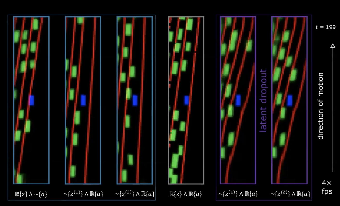
Figure 18: Performance with latent dropout

In the last two images on the right-hand side, we see two different sets of latent variables having a real sequence of actions and these networks have been trained with the latent dropout trick. We can now see that the rotation is now encoded by the action and no longer by the latent variables.

Training the agent

In the previous sections, we saw how we can obtain a world model by simulating real world experiences. In this section, we will use this world model to train our agent. Our goal is to learn the policy to take an action given the history of previous states. Given a state $s_t$ (velocity, position & context images), the agent takes an action $a_t$ (acceleration, brake & steering), the world model outputs a next state and cost associated with that $(s_t, a_t)$ pair which is a combination of proximity cost and lane cost.

As discussed in the previous section, to avoid hazy predictions, we need to sample latent variable $z_t$ from the encoder module of the future state $s_{t+1}$ or from prior distribution $P(z)$. The world model gets previous states $s_{1:t}$, action taken by our agent and latent variable $z_t$ to predict the next state $\hat s_{t+1}$ and the cost. This constitutes one module that is replicated multiple times (Figure 19) to give us final prediction and loss to optimize.

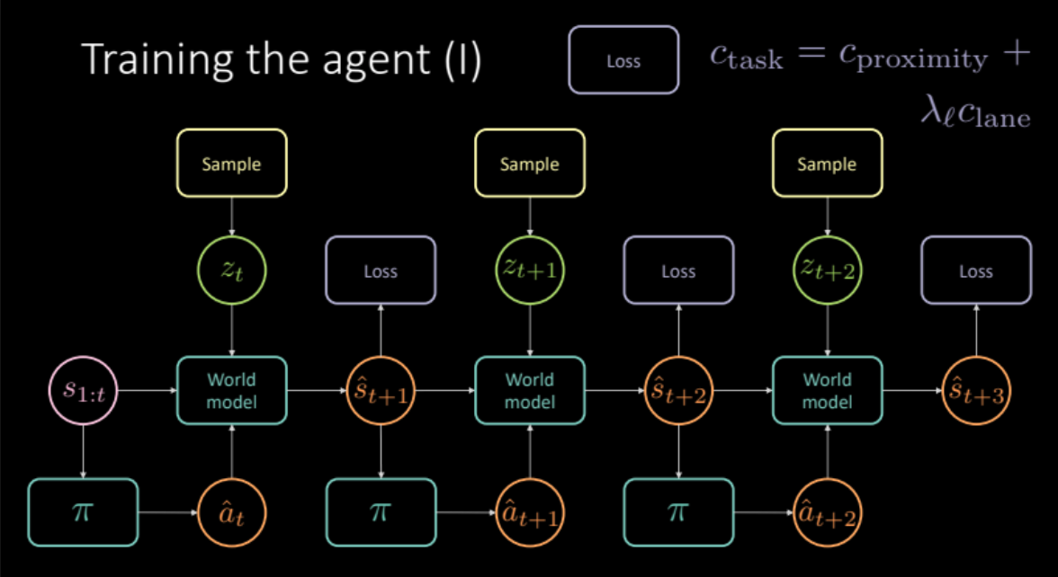
Figure 19: Task specific model architecture

So, we have our model ready. Let’s see how it looks !!

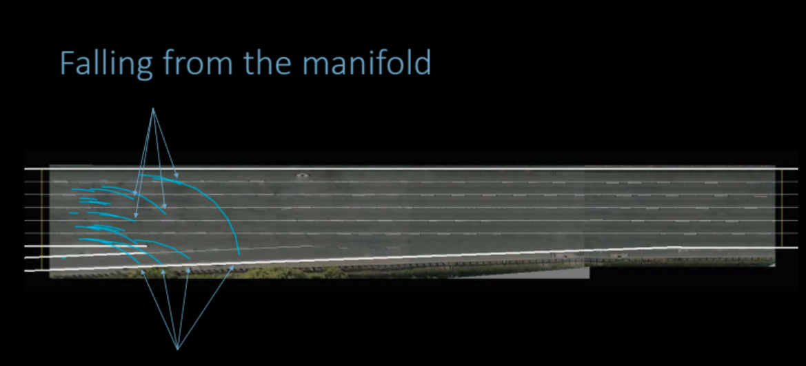
Figure 20: Learned policy: Agent either collides or moves away from the road

Unfortunately, this does not work. Policy trained this way is not useful as it learns to predict all black since it results in zero cost.

How can we address this issue? Can we try imitating other vehicles to improve our predictions?

Imitating the expert

How do we imitate the experts here? We want the prediction of our model after taking a particular action from a state to be as close as possible to the actual future. This acts as an expert regulariser for our training. Our cost function now includes both the task specific cost(proximity cost and lane cost) and this expert regulariser term. Now as we are also calculating the loss with respect to the actual future, we have to remove the latent variable from the model because the latent variable gives us a specific prediction, but this setting works better if we just work with the average prediction.

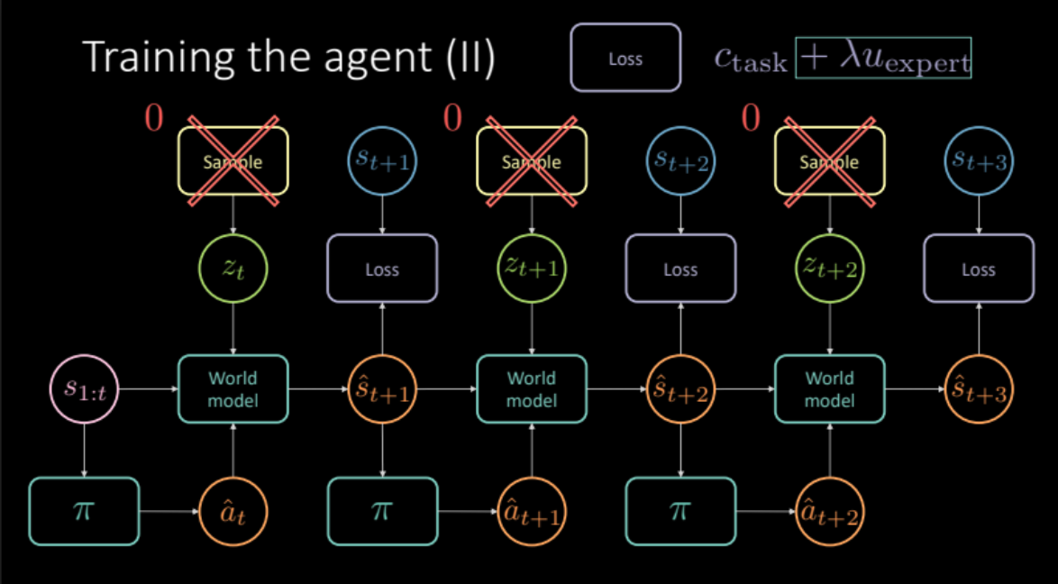
Figure 21: Expert regularization based model architecture

So how does this model perform?

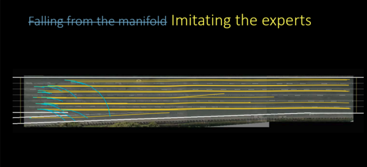
Figure 22: Learned policy by imitating the experts

As we can see in the above figure, the model actually does incredibly well and learns to make very good predictions. This was model based imitation learning, we tried to model our agent to try to imitate others.

But can we do better? Did we just train the Variational Autoencoder to remove it in the end?

It turns out we can still improve if we look to minimize the uncertainty of the forward model predictions.

Minimizing the Forward Model Uncertainty

What do we mean by minimizing forward model uncertainty and how would we do it? Before we answer that, let’s recap something we saw in the third week’s practicum.

If we train multiple models on the same data, all those models agree on the points in the training region (shown in red) resulting in zero variance in the training region. But as we move further away from the training region, the trajectories of loss functions of these models start diverging and variance increases. This is depicted in the figure 23. But as the variance is differentiable, we can run gradient descent over the variance in order to minimize it.

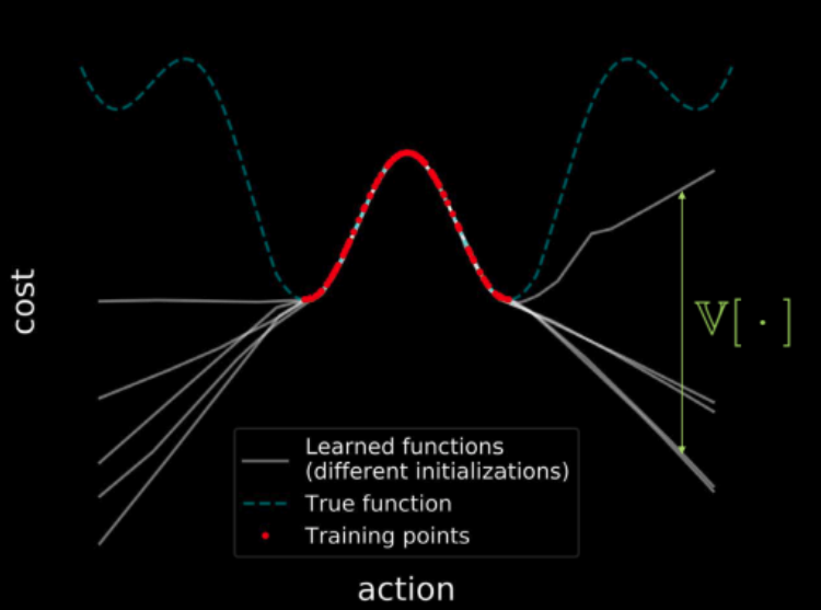
Figure 23: Cost visualization across the entire input space

Coming back to our discussion, we observe that learning a policy using only observational data is challenging because the distribution of states it produces at execution time may differ from what was observed during the training phase. The world model may make arbitrary predictions outside the domain it was trained on, which may wrongly result in low cost. The policy network may then exploit these errors in the dynamics model and produce actions which lead to wrongly optimistic states.

To address this, we propose an additional cost which measures the uncertainty of the dynamics model about its own predictions. This can be calculated by passing the same input and action through several different dropout masks, and computing the variance across the different outputs. This encourages the policy network to only produce actions for which the forward model is confident.

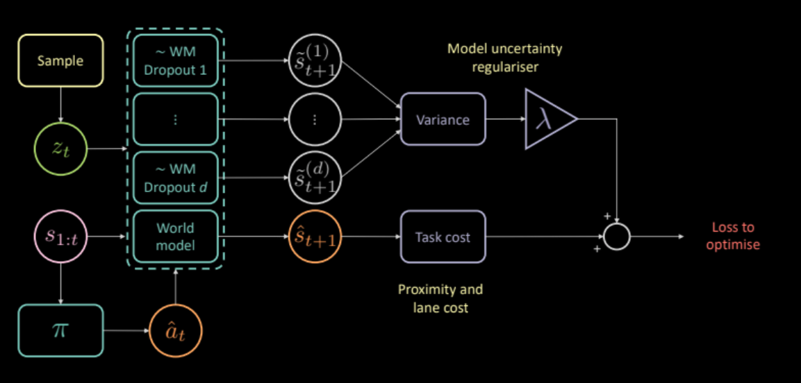
Figure 24: Uncertainty regulariser based model architecture

So, does uncertainty regulariser help us in learning better policy?

Yes, it does. The policy learned this way is better than the previous models.

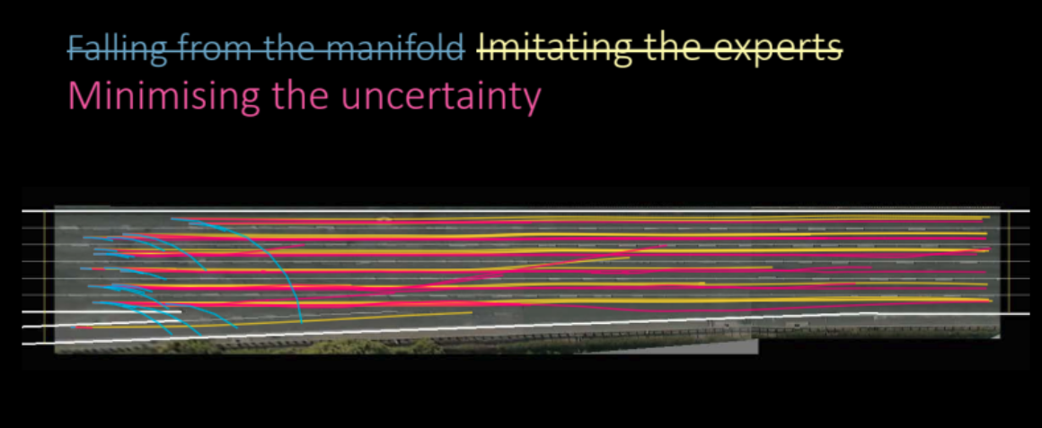
Figure 25: Learned policy based on uncertainty regulariser

Evaluation

Figure 26 shows how well our agent learned to drive in dense traffic. Yellow car is the original driver, blue car is our learned agent and all green cars are blind to us (cannot be controlled).

Figure 26: Performance of model with uncertainty regulariser