The Truck Backer-Upper

Setup

The goal of this task is to build a self-learning controller which controls the steering of the truck while it backs up to the loading dock from any arbitrary initial position.

Note that only backing up is allowed, as shown below in Figure 1.

Fig. 1: The Truck, Trailer and Loading Dock

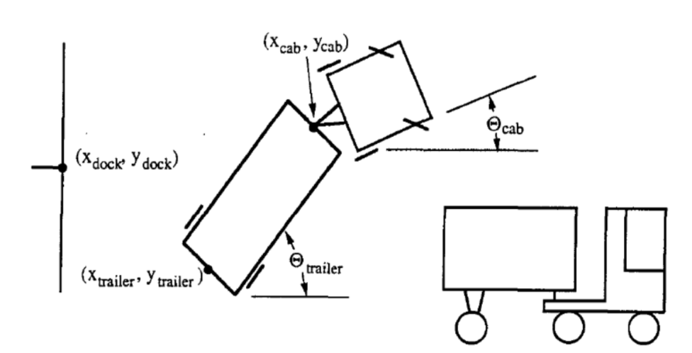The state of the truck is represented by six parameters:

• $\tcab$: Angle of the truck
• $\xcab, \ycab$: The cartesian of the yoke (or front of the trailer).
• $\ttrailer$: Angle of the trailer
• $\xtrailer, \ytrailer$: The cartesian of the (back of the) trailer.

The goal of the controller is to select an appropriate angle $\phi$ at each time $k$, where after the truck will back up in a fixed small distance. Success depends on two criteria:

1. The back of the trailer is parallel to the wall loading dock, e.g. $\ttrailer = 0$.
2. The back of the trailer ($\xtrailer, \ytrailer$) is as close as possible to the point ($x_{dock}, y_{dock}$) as shown above.

More Parameters and Visualization

Fig. 2: Parameters for visualization

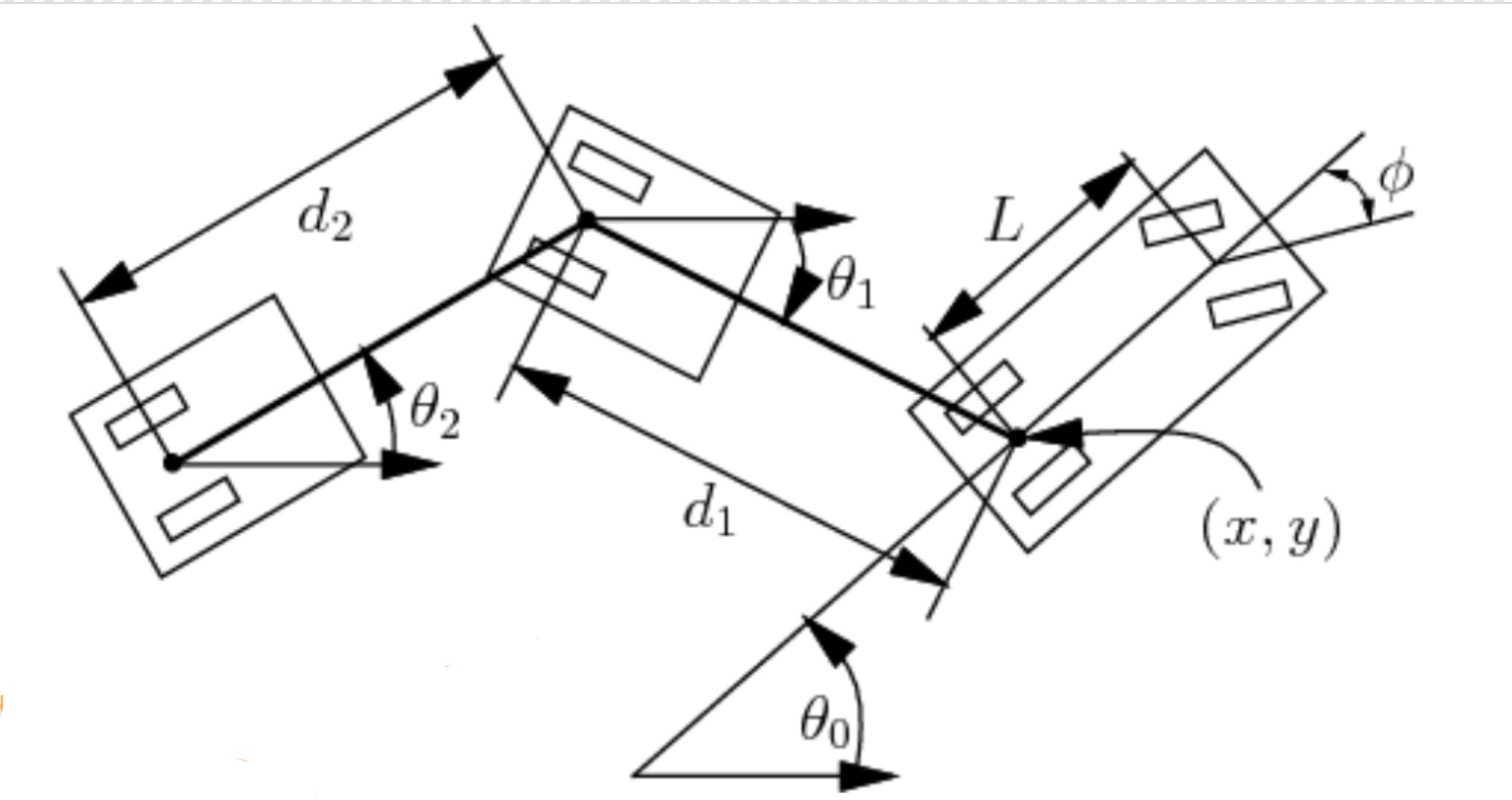In this section, we also consider a few more parameters shown in Figure 2. Given car length $L$, $d_1$ the distance between car and trailer and $d_2$ the length of the trailer, etc, we can calculate the change of angle and positions:

Here, $s$ denotes the signed speed and $\phi$ the negative steering angle. Now we can represent the state by only four parameters: $\xcab$, $\ycab$, $\theta_0$ and $\theta_1$. This is because Length parameters are known and $\xtrailer, \ytrailer$ is determined by $\xcab, \ycab, d_1, \theta_1$.

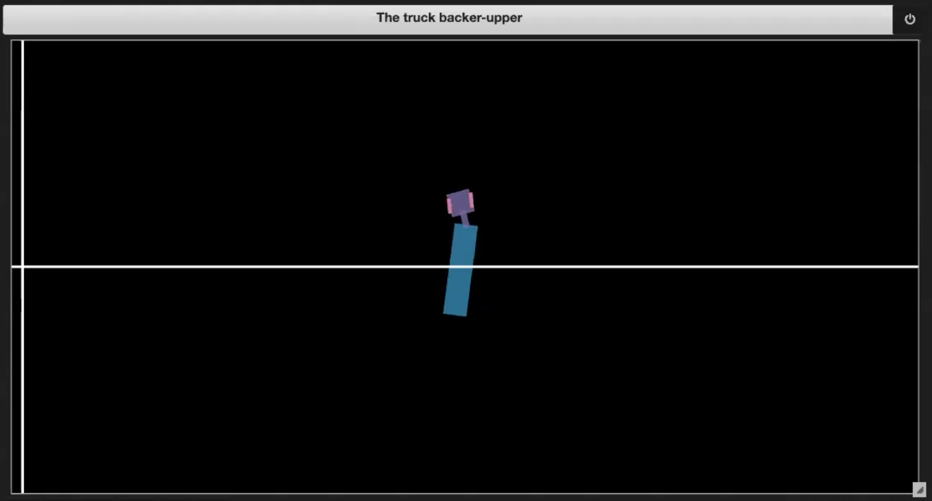
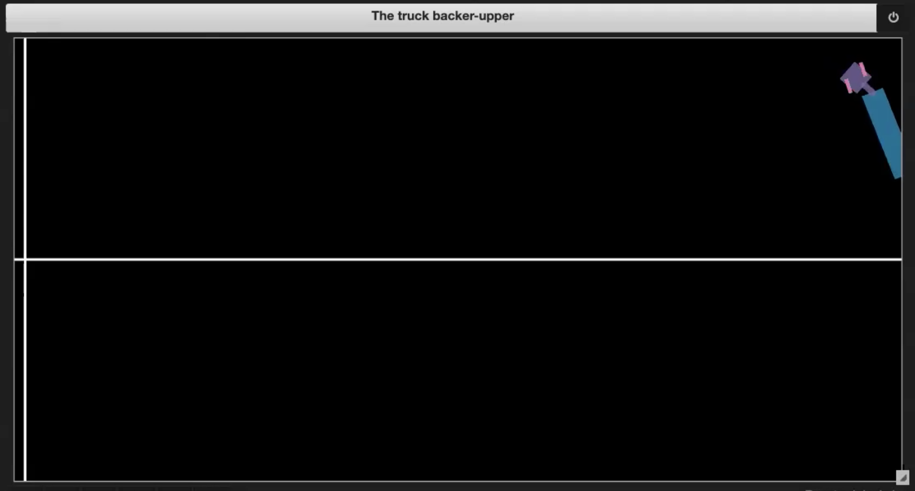
In the Jupyter Notebook from the Deep Learning repository, we have some sample environments shown in Figures 3.(1-4):

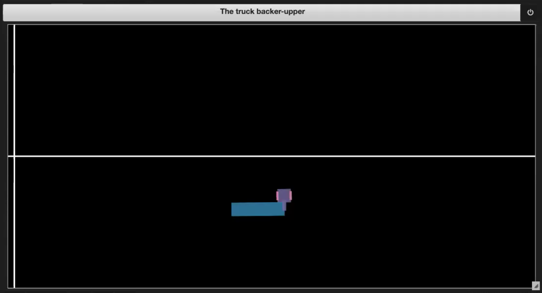Fig. 3.1: Sample plot of the environment	Fig. 3.2: Driving into itself (jackknifing)
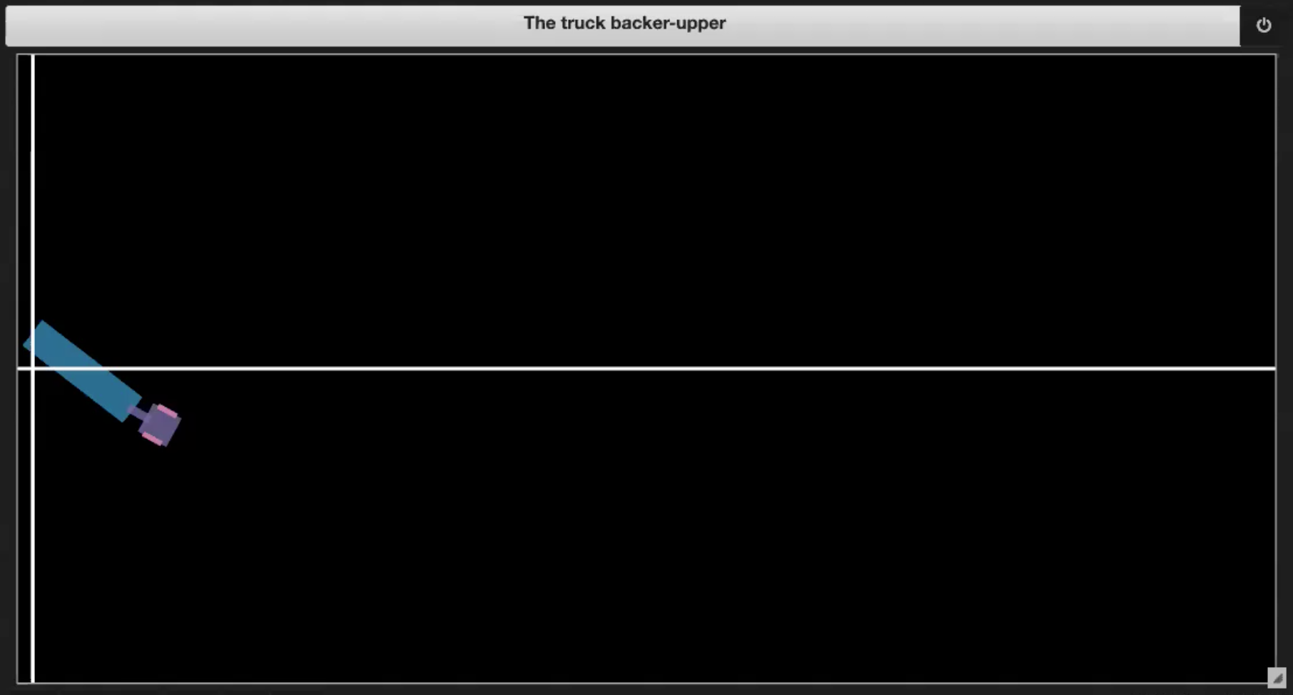Fig. 3.3: Going out of boundary	Fig. 3.4: Reaching the dock

At each time step $k$, a steering signal which ranges from $-\frac{\pi}{4}$ to $\frac{\pi}{4}$ will be fed in and the truck will take back up using the corresponding angle.

There are several situations where the sequence can end:

• If the truck drives into itself (jackknifes, as in Figure 3.2)
• If the truck goes out of boundary (shown in Figure 3.3)
• If the truck reaches the dock (shown in Figure 3.4)

Training

The training process involves two stages: (1) training of a neural network to be an emulator of the truck and trailer kinematics and (2) training of a neural network controller to control the truck.

Fig. 4: Overview Diagram

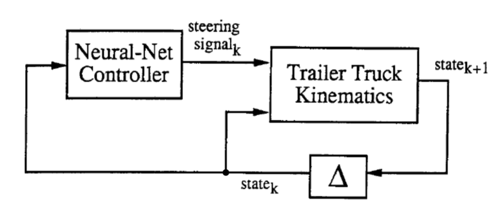As shown above, in the abstract diagram, the two blocks are the two networks that will be trained. At each time step $k$, the “Trailer Truck Kinematics”, or what we have been calling the emulator, takes in the 6-dimension state vector and the steering signal generated from the controller and generate a new 6-dimension state at time $k + 1$.

Emulator

The emulator takes the current location ($\tcab^t$,$\xcab^t, \ycab^t$, $\ttrailer^t$, $\xtrailer^t$, $\ytrailer^t$) plus the steering direction $\phi^t$ as input and outputs the state at next timestep ($\tcab^{t+1}$,$\xcab^{t+1}, \ycab^{t+1}$, $\ttrailer^{t+1}$, $\xtrailer^{t+1}$, $\ytrailer^{t+1}$). It consists of a linear hidden layer, with ReLu activation function, and an linear output layer. We use MSE as the loss function and train the emulator via stochastic gradient descent.

Fig. 5: Training the Neural-net Emulator

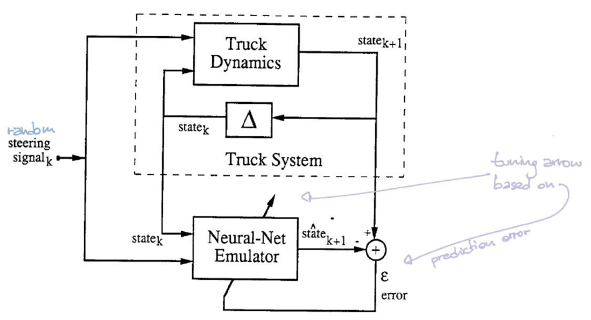In this setup, the the simulator can tell us the location of next step given the current location and steering angle. Therefore, we don’t really need a neural-net that emulates the simulator. However, in a more complex system, we may not have access to the underlying equations of the system, i.e. we do not have the laws of the universe in a nice computable form. We may only observe data that records sequences of steering signals and their corresponding paths. In this case, we want to train a neural-net to emulate the dynamic of this complex system.

In order to train enumlator, there are two important function in Class truck we need to look into when we train the emulator.

First is the step function which gives the output state of the truck after computation.

def step(self, ϕ=0, dt=1):

    # Check for illegal conditions
    if self.is_jackknifed():
        print('The truck is jackknifed!')
        return

    if self.is_offscreen():
        print('The car or trailer is off screen')
        return

    self.ϕ = ϕ
    x, y, W, L, d, s, θ0, θ1, ϕ = self._get_atributes()

    # Perform state update
    self.x += s * cos(θ0) * dt
    self.y += s * sin(θ0) * dt
    self.θ0 += s / L * tan(ϕ) * dt
    self.θ1 += s / d * sin(θ0 - θ1) * dt

Second is the state function which gives the current state of the truck.

def state(self):
        return (self.x, self.y, self.θ0, *self._traler_xy(), self.θ1)

We generate two lists first. We generate an input list by appending the randomly generated steering angle ϕ and the initial state which coming from the truck by running truck.state(). And we generate an output list that is appended by the output state of the truck which can be computed by truck.step(ϕ).

We now can train the emulator:

cnt = 0
for i in torch.randperm(len(train_inputs)):
    ϕ_state = train_inputs[i]
    next_state_prediction = emulator(ϕ_state)

    next_state = train_outputs[i]
    loss = criterion(next_state_prediction, next_state)

    optimiser_e.zero_grad()
    loss.backward()
    optimiser_e.step()

    if cnt == 0 or (cnt + 1) % 1000 == 0:
        print(f'{cnt + 1:4d} / {len(train_inputs)}, {loss.item():.10f}')
    cnt += 1

Notice that torch.randperm(len(train_inputs)) gives us a random permutation of the indices within the range $0$ to length of training inputs minus $1$. After the permutation of indices, each time ϕ_state is chosen from the input list at the index i. We input ϕ_state through the emulator function that has a linear output layer and we get next_state_prediction. Notice that the emulator is a neural netork defined as below:

emulator = nn.Sequential(
    nn.Linear(steering_size + state_size, hidden_units_e),
    nn.ReLU(),
    nn.Linear(hidden_units_e, state_size)
)

Here we use MSE to calculate the loss between the true next state and the next state prediction, where the true next state is coming from the output list with index i that corresponding to the index of the ϕ_state from input list.

Controller

Refer to Figure 5. Block $\matr{C}$ represents the controller. It takes in the current state and ouputs a steering angle. Then block $\matr{T}$ (emulator) takes both the state and angle to produce the next state.

Fig. 5: State Transition flow diagram

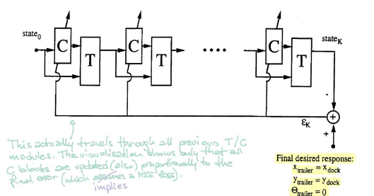To train the controller, we start from a random initial state and repeat the procedure($\matr{C}$ and $\matr{T}$) until the trailer is parallel to the dock. The error is calculated by comparing the trailer location and dock location. We then find the gradients using backpropagation and update parameters of the controller via SGD.

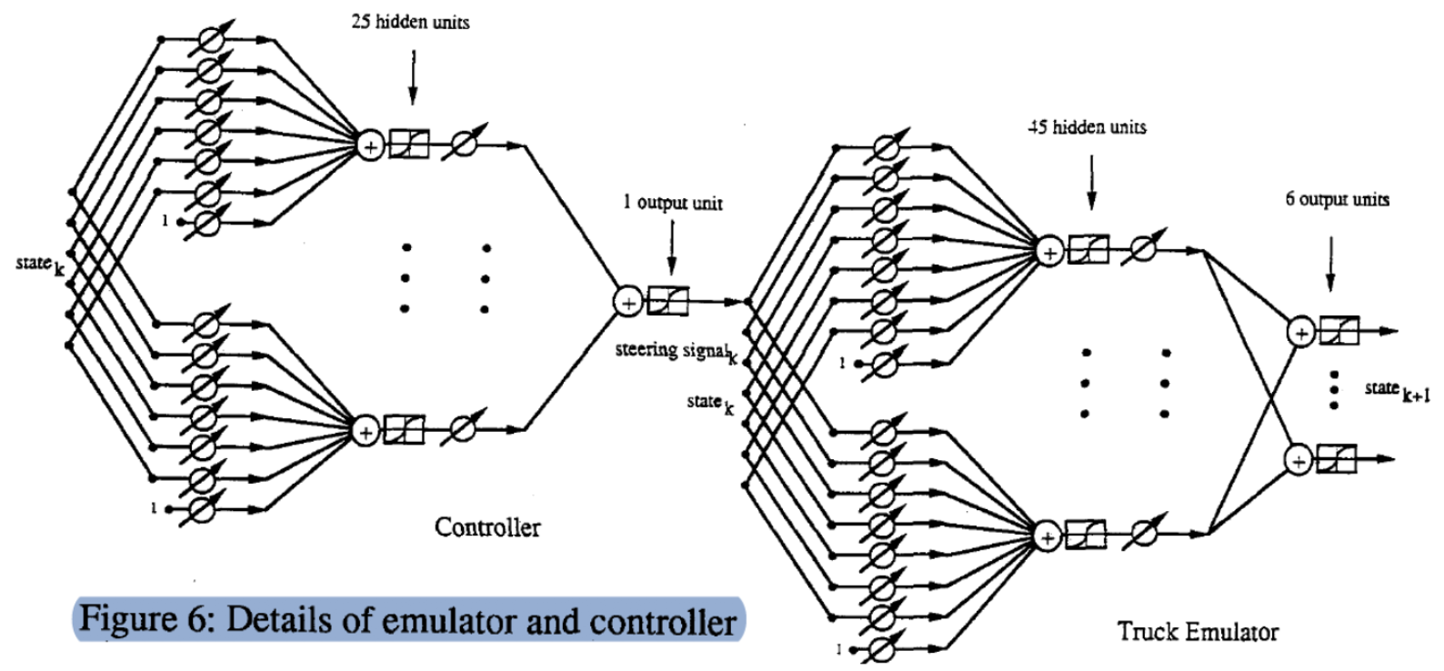
Detailed Model Structure

This is a detailed graph of ($\matr{C}$, $\matr{T}$) process. We start with a state (6 dimension vector), multiply it with a tunable weights matrix and get 25 hidden units. Then we pass it through another tunable weights vector to get the output (steering signal). Similarly, we input the state and angle $\phi$ (7 dimension vector) through two layers to produce the state of next step.

To see this more clearly, we show the exact implementation of the emulator:

state_size = 6
steering_size = 1
hidden_units_e = 45

emulator = nn.Sequential(
    nn.Linear(steering_size + state_size, hidden_units_e),
    nn.ReLU(),
    nn.Linear(hidden_units_e, state_size)
)

optimiser_e = SGD(emulator.parameters(), lr=0.005)
criterion = nn.MSELoss()

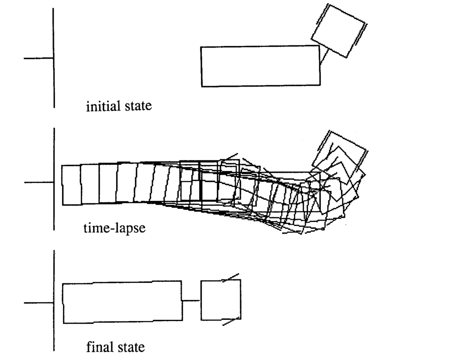
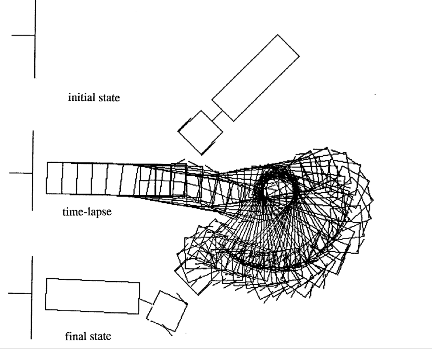
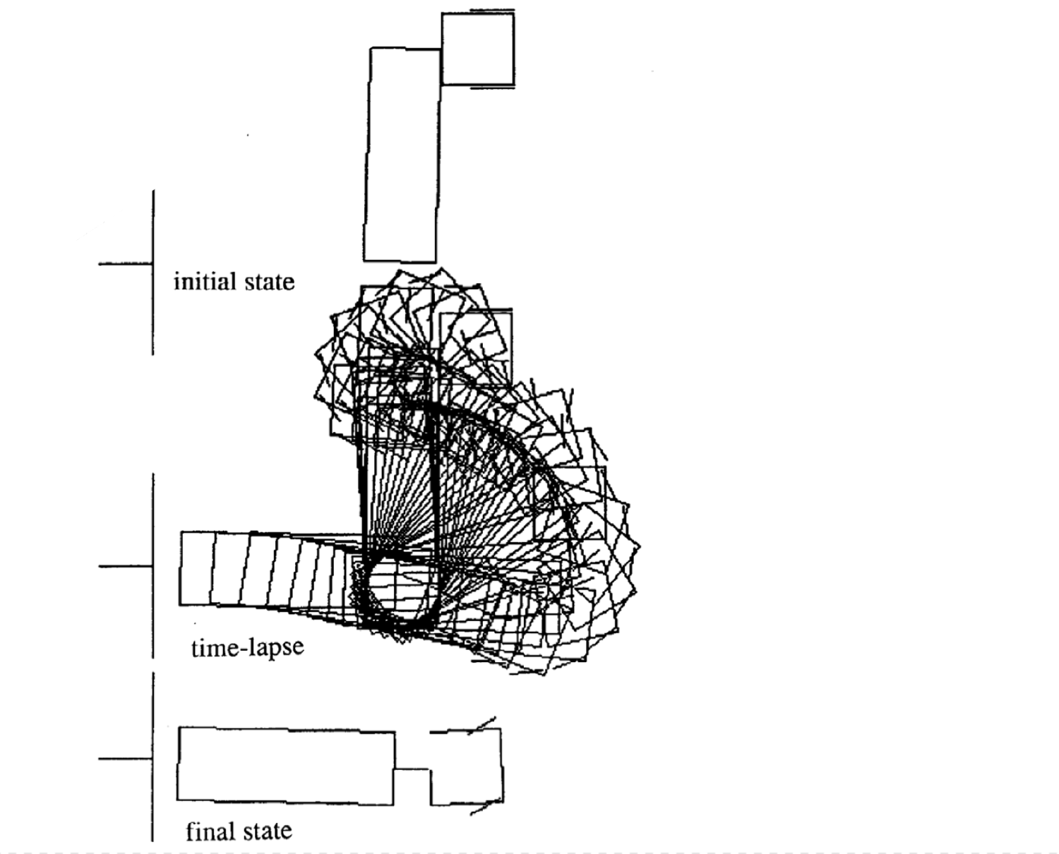
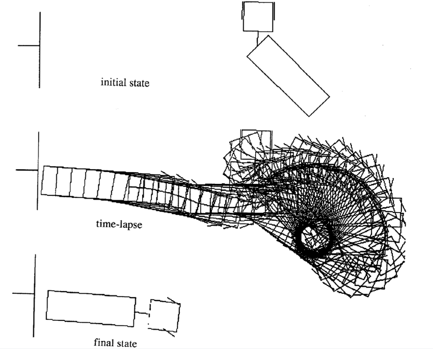
Examples of Movement

Following are four examples of movement for different initial state. Notice that the number of time steps in each episode varies.

Fig. 7: Examples of movement for four different initial states

Additional Resources:

A full working demo can be found at: https://tifu.github.io/truck_backer_upper/. Please check out the code as well, which can be found at https://github.com/Tifu/truck_backer_upper.