Self-Supervised Learning - ClusterFit and PIRL

What is missing from “pretext” tasks? The hope of generalization

Pretext task generally comprises of pretraining steps which is self-supervised and then we have our transfer tasks which are often classification or detection. We hope that the pretraining task and the transfer tasks are “aligned”, meaning, solving the pretext task will help solve the transfer tasks very well. So, a lot of research goes into designing a pretext task and implementing them really well.

However, it is very unclear why performing a non-semantic task should produce good features?. For example, why should we expect to learn about “semantics” while solving something like Jigsaw puzzle? Or why should “predicting hashtags” from images be expected to help in learning a classifier on transfer tasks? Therefore, the question remains. How should we design good pre-training tasks which are well aligned with the transfer tasks?

One way to evaluate this problem is by looking at representations at each layer (refer Fig. 1). If the representations from the last layer are not well aligned with the transfer task, then the pretraining task may not be the right task to solve.

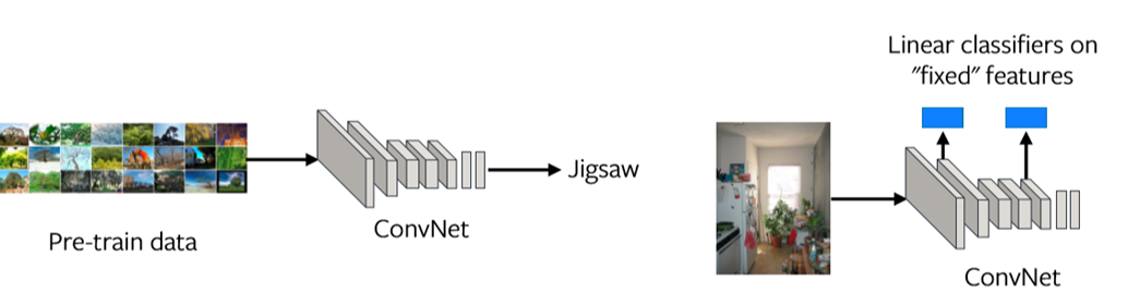
Fig. 1: Feature representations at each layer

Fig. 2 plots the Mean Average Precision at each layer for Linear Classifiers on VOC07 using Jigsaw Pretraining. It is clear that the last layer is very specialized for the Jigsaw problem.

Fig. 2: Performance of Jigsaw based on each layer

What we want from pre-trained features?

• Represent how images relate to one another

  • ClusterFit: Improving Generalization of Visual Representations

• Be robust to “nuisance factors” – Invariance

  E.g. exact location of objects, lighting, exact colour

  • PIRL: Self-supervised learning of Pre-text Invariant Representations

Two ways to achieve the above properties are Clustering and Contrastive Learning. They have started performing much better than whatever pretext tasks that were designed so far. One method that belongs to clustering is ClusterFit and another falling into invariance is PIRL.

ClusterFit: Improving Generalization of Visual Representations

Clustering the feature space is a way to see what images relate to one another.

Method

ClusterFit follows two steps. One is the cluster step, and the other is the predict step.

Cluster: Feature Clustering

We take a pretrained network and use it to extract a bunch of features from a set of images. The network can be any kind of pretrained network. K-means clustering is then performed on these features, so each image belongs to a cluster, which becomes its label.

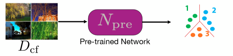
Fig. 3: Cluster step

Fit: Predict Cluster Assignment

For this step, we train a network from scratch to predict the pseudo labels of images. These pseudo labels are what we obtained in the first step through clustering.

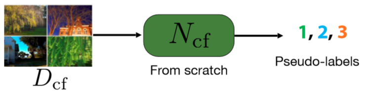
Fig. 4: Predict step

A standard pretrain and transfer task first pretrains a network and then evaluates it in downstream tasks, as it is shown in the first row of Fig. 5. ClusterFit performs the pretraining on a dataset $D_{cf}$ to get the pretrained network $N_{pre}$. The pretrained network $N_{pre}$ are performed on dataset $D_{cf}$ to generate clusters. We then learn a new network $N_{cf}$from scratch on this data. Finally, use $N_{cf}$ for all downstream tasks.

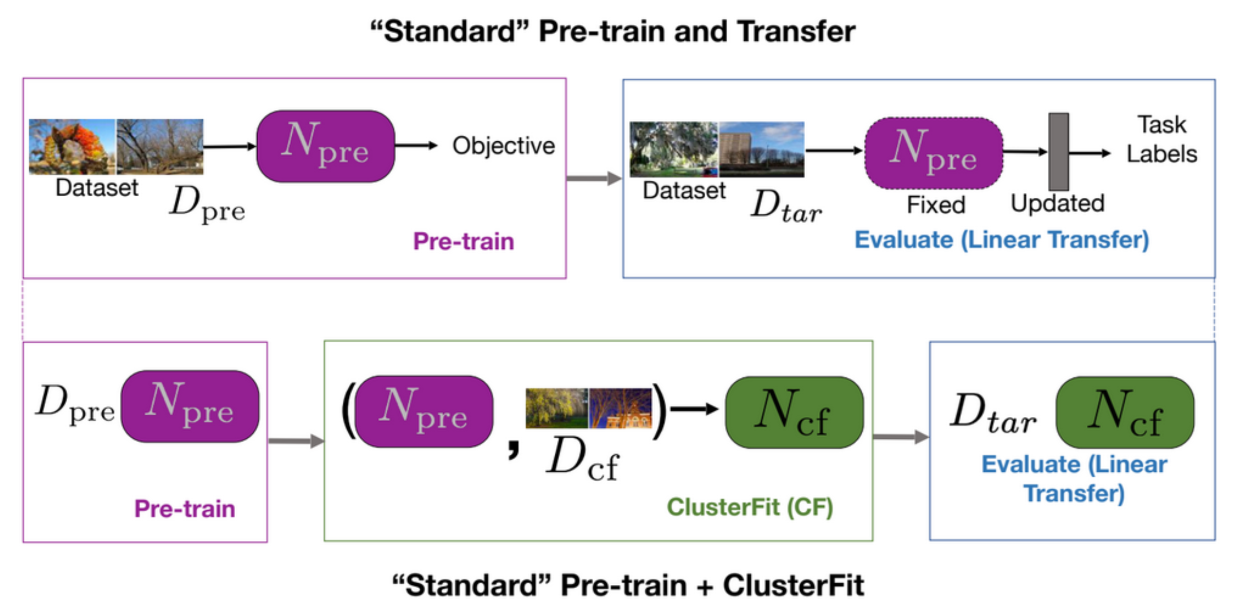
Fig. 5: "Standard" pretrain + transfer *vs.* "Standard" pretrain + ClusterFit

Why ClusterFit Works

The reason why ClusterFit works is that in the clustering step only the essential information is captured, and artefacts are thrown away making the second network learn something slightly more generic.

To understand this point, a fairly simple experiment is performed. We add label noise to ImageNet-1K, and train a network based on this dataset. Then, we evaluate the feature representation from this network on a downstream task on ImageNet-9K. As it is shown in Fig. 6, we add different amounts of label noise to the ImageNet-1K, and evaluate the transfer performance of different methods on ImageNet-9K.

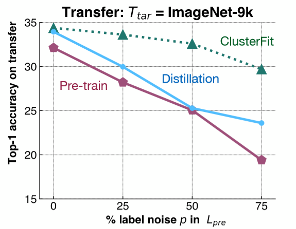
Fig. 6: Control Experiment

The pink line shows the performance of pretrained network, which decreases as the amount of label noise increases. The blue line represents model distillation where we take the initial network and use it to generate labels. Distillation generally performs better than pretrained network. The green line, ClusterFit, is consistently better than either of these methods. This result validates our hypothesis.

• Question: Why use distillation method to compare. What’s the difference between distillation and ClusterFit?

In model distillation we take the pre-trained network and use the labels the network predicted in a softer fashion to generate labels for our images. For example, we get a distribution over all the classes and use this distribution to train the second network. The softer distribution helps enhance the initial classes that we have. In ClusterFit we don’t care about the label space.

Performance

We apply this method to self-supervised learning. Here Jigsaw is applied to obtain the pretrained network $N_{pre}$ in ClusterFit. From Fig. 7 we see that the transfer performance on different datasets shows a surprising amount of gains, compared to other self-supervised methods.

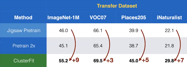
Fig. 7: Transfer performance on different datasets

ClusterFit works for any pre-trained network. Gains without extra data, labels or changes in architecture can be seen in Fig. 8. So in some way, we can think of the ClusterFit as a self-supervised fine-tuning step, which improves the quality of representation.

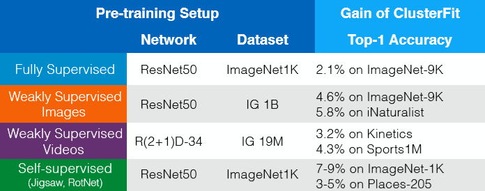
Fig. 8: Gains without extra data, labels or changes in architecture

Self-supervised Learning of Pretext Invariant Representations (PIRL)

Contrastive Learning

Contrastive learning is basically a general framework that tries to learn a feature space that can combine together or put together points that are related and push apart points that are not related.

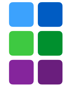
Fig. 9: Groups of Related and Unrelated Images

In this case, imagine like the blue boxes are the related points, the greens are related, and the purples are related points.

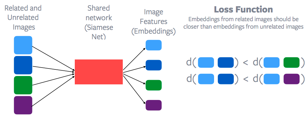
Fig. 10: Contrastive Learning and Loss Function

Features for each of these data points would be extracted through a shared network, which is called Siamese Network to get a bunch of image features for each of these data points. Then a contrastive loss function is applied to try to minimize the distance between the blue points as opposed to, say, the distance between the blue point and the green point. Or the distance basically between the blue points should be less than the distance between the blue point and green point or the blue point and the purple point. So, embedding space from the related samples should be much closer than embedding space from the unrelated samples. So that’s the general idea of what contrastive learning is and of course Yann was one of the first teachers to propose this method. So contrastive learning is now making a resurgence in self-supervised learning pretty much a lot of the self-supervised state of the art methods are really based on contrastive learning.

How to define related or unrelated?

And the main question is how to define what is related and unrelated. In the case of supervised learning that’s fairly clear all of the dog images are related images, and any image that is not a dog is basically an unrelated image. But it’s not so clear how to define the relatedness and unrelatedness in this case of self-supervised learning. The other main difference from something like a pretext task is that contrastive learning really reasons a lot of data at once. If you look at the loss function, it always involves multiple images. In the first row it involves basically the blue images and the green images and in the second row it involves the blue images and the purple images. But as if you look at a task like say Jigsaw or a task like rotation, you’re always reasoning about a single image independently. So that’s another difference with contrastive learning: contrastive learning reasons about multiple data points at once.

Similar techniques to what was discussed earlier could be used: frames of video or sequential nature of data. Frames that are nearby in a video are related and frames, say, from a different video or which are further away in time are unrelated. And that has formed the basis of a lot of self- supervised learning methods in this area. This method is called CPC, which is contrastive predictive coding, which relies on the sequential nature of a signal and it basically says that samples that are close by, like in the time-space, are related and samples that are further apart in the time-space are unrelated. A fairly large amount of work basically exploiting this: it can either be in the speech domain, video, text, or particular images. And recently, we’ve also been working on video and audio so basically saying a video and its corresponding audio are related samples and video and audio from a different video are basically unrelated samples.

Tracking Objects

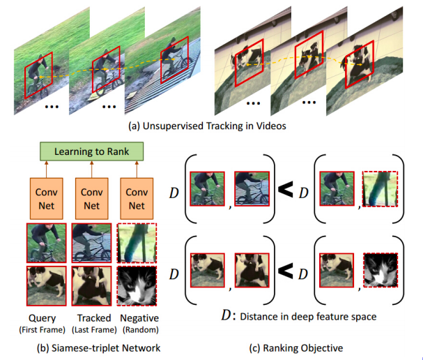
Fig. 11: Tracking the Objects

Some of the early work, like self-supervised learning, also uses this contrastive learning method and they really defined related examples fairly interestingly. You run a tracked object tracker over a video and that gives you a moving patch and what you say is that any patch that was tracked by the tracker is related to the original patch. Whereas, any patch from a different video is not a related patch. So that basically gives out these bunch of related and unrelated samples. In figure 11(c), you have this like distance notation. What this network tries to learn is basically that patches that are coming from the same video are related and patches that are coming from different videos are not related. In some way, it automatically learns about different poses of an object. It tries to group together a cycle, viewed from different viewing angles or different poses of a dog.

Nearby patches vs. distant patches of an Image

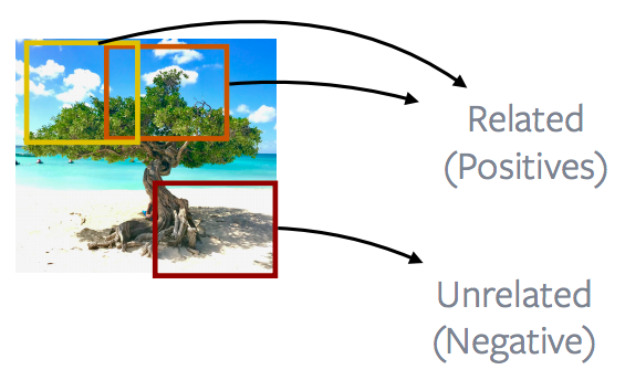
Fig. 12: Nearby patches *vs.* distant patches of an Image

In general, talking about images, a lot of work is done on looking at nearby image patches versus distant patches, so most of the CPC v1 and CPC v2 methods are really exploiting this property of images. So image patches that are close are called as positives and image patches that are further apart are translated as negatives, and the goal is to minimize the contrastive loss using this definition of positives and negatives.

Patches of an image vs. patches of other images

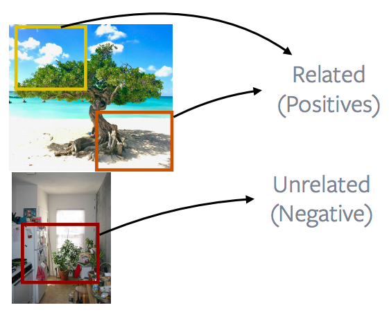
Fig. 13: Patches of an Image *vs.* Patches of Other Images

The more popular or performant way of doing this is to look at patches coming from an image and contrast them with patches coming from a different image. This forms the basis of a lot of popular methods like instance discrimination, MoCo, PIRL, SimCLR. The idea is basically what’s shown in the image. To go into more details, what these methods do is to extract completely random patches from an image. These patches can be overlapping, they can actually become contained within one another or they can be completely falling apart and then apply some data augmentation. In this case, say, a colour chattering or removing the colour or so on. And then these two patches are defined to be positive examples. Another patch is extracted from a different image. And this is again a random patch and that basically becomes your negatives. And a lot of these methods will extract a lot of negative patches and then they will basically perform contrastive learning. So there are relating two positive samples, but there are a lot of negative samples to do contrastive learning against.

Underlying Principle for Pretext Tasks

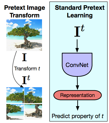
Fig. 14: Pretext Image Transform and Standard Pretext Learning

Now moving to PIRL a little bit, and that’s trying to understand what the main difference of pretext tasks is and how contrastive learning is very different from the pretext tasks. Again, pretext tasks always reason about a single image at once. So the idea is that given an image your and prior transform to that image, in this case a Jigsaw transform, and then inputting this transformed image into a ConvNet and trying to predict the property of the transform that you applied to, the permutation that you applied or the rotation that you applied or the kind of colour that you removed and so on. So the pretext tasks always reason about a single image. And the second thing is that the task that you’re performing in this case really has to capture some property of the transform. So it really needs to capture the exact permutation that are applied or the kind of rotation that are applied, which means that the last layer representations are actually going to go PIRL very a lot as the transform the changes and that is by design, because you’re really trying to solve that pretext tasks. But unfortunately, what this means is that the last layer representations capture a very low-level property of the signal. They capture things like rotation or so on. Whereas what is designed or what is expected of these representations is that they are invariant to these things that it should be able to recognize a cat, no matter whether the cat is upright or that the cat is say, bent towards like by 90 degrees. Whereas when you’re solving that particular pretext task you’re imposing the exact opposite thing. We’re saying that we should be able to recognize whether this picture is upright or whether this picture is basically turning it sideways. There are many exceptions in which you really want these low-level representations to be covariant and a lot of it really has to do with the tasks that you’re performing and quite a few tasks in 3D really want to be predictive. So you want to predict what camera transforms you have: you’re looking at two views of the same object or so on. But unless you have that kind of a specific application for a lot of semantic tasks, you really want to be invariant to the transforms that are used to use that input.

How important has invariance been?

Invariance has been the word course for feature learning. Something like SIFT, which is a fairly popular handcrafted feature where we inserted here is transferred invariant. And supervise networks, for example, supervised Alex nets, they’re trained to be invariant data augmentation. You want this network to classify different crops or different rotations of this image as a tree, rather than ask it to predict what exactly was the transformation applied for the input.

PIRL

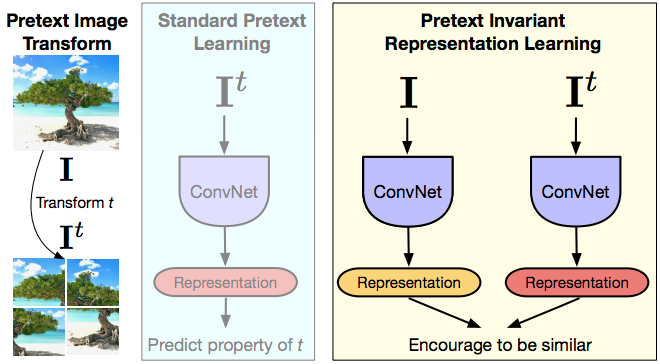
Fig. 15: PIRL

This is what inspired PIRL. So PIRL stands for pretext invariant representation learning, where the idea is that you want the representation to be invariant or capture as little information as possible of the input transform. So you have the image, you have the transformed version of the image, you feed-forward both of these images through a ConvNet, you get a representation and then you basically encourage these representations to be similar. In terms of the notation referred earlier, the image $I$ and any pretext transformed version of this image $I^t$ are related samples and any other image is underrated samples. So in this way when you frame this network, representation hopefully contains very little information about this transform $t$. And assume you are using contrastive learning. So the contrastive learning part is basically you have the saved feature $v_I$ coming from the original image $I$ and you have the feature $v_{I^t}$ coming from the transform version and you want both of these representations to be the same. And the book paper we looked at is two different states of the art of the pretext transforms, which is the jigsaw and the rotation method discussed earlier. In some way, this is like multitask learning, but just not really trying to predict both designed rotation. You’re trying to be invariant of Jigsaw rotation.

Using a Large Number of Negatives

The key thing that has made contrastive learning work well in the past, taking successful attempts is using a large number of negatives. One of the good paper taking successful attempts, is instance discrimination paper from 2018, which introduced this concept of a memory bank. This is powered, most of the research methods which are state of the art techniques hinge on this idea for a memory bank. The memory bank is a nice way to get a large number of negatives without really increasing the sort of computing requirement. What you do is you store a feature vector per image in memory, and then you use that feature vector in your contrastive learning.

How it works

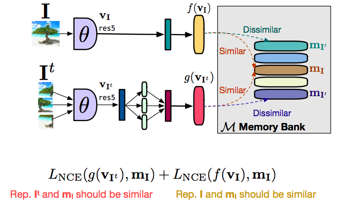
Fig. 16: How does the Memory Bank Work

Let’s first talk about how you would do this entire PIRL setup without using a memory bank. So you have an image $I$ and you have an image $I^t$, and you feed-forward both of these images, you get a feature vector $f(v_I)$ from the original image $I$, you get a feature $g(v_{I^t})$ from the transform versions, the patches, in this case. What you want is the features $f$ and $g$ to be similar. And you want features from any other unrelated image to basically be dissimilar. In this case, what we can do now is if you want a lot of negatives, we would really want a lot of these negative images to be feed-forward at the same time, which really means that you need a very large batch size to be able to do this. Of course, a large batch size is not really good, if not possible, on a limited amount of GPU memory. The way to do that is to use something called a memory bank. So what this memory bank does is that it stores a feature vector for each of the images in your data set, and when you’re doing contrastive learning rather than using feature vectors, say, from a different from a negative image or a different image in your batch, you can just retrieve these features from memory. You can just retrieve features of any other unrelated image from the memory and you can just substitute that to perform contrastive learning. Simply dividing the objective into two parts, there was a contrasting term to bring the feature vector from the transformed image $g(v_I)$, similar to the representation that we have in the memory so $m_I$. And similarly, we have a second contrastive term that tries to bring the feature $f(v_I)$ close to the feature representation that we have in memory. Essentially $g$ is being pulled close to $m_I$ and $f$ is being pulled close to $m_I$. By transitivity, $f$ and $g$ are being pulled close to one another. And the reason for separating this out was that it stabilized training and we were not able to train without doing this. Basically, the training would not really converge. By separating this out into two forms, rather than doing direct contrastive learning between $f$ and $g$, we were able to stabilize training and actually get it working.

PIRL Pre-training

The way to evaluate this is basically by standard pre-training evaluation set-up. For transfer learning, we can pretrain on images without labels. The standard way of doing this is to take an image net, throw away the labels and pretend as unsupervised.

Evaluation

Evaluation can be performed by full fine-tuning (initialisation evaluation) or training a linear classifier (feature evaluation). PIRL robustness has been tested by using images in-distribution by training it on in-the-wild images. So we just took 1 million images randomly from Flickr, which is the YFCC data set. And then we basically performed pre-training on these images and then performed transplanting on different data sets.

Evaluating on Object Detection task

PIRL was first evaluated on object detection task (a standard task in vision) and it was able to outperform ImageNet supervised pre-trained networks on both VOC07+12 and VOC07 data sets. In fact, PIRL outperformed even in the stricter evaluation criteria, $AP^{all}$ and that’s a good positive sign.

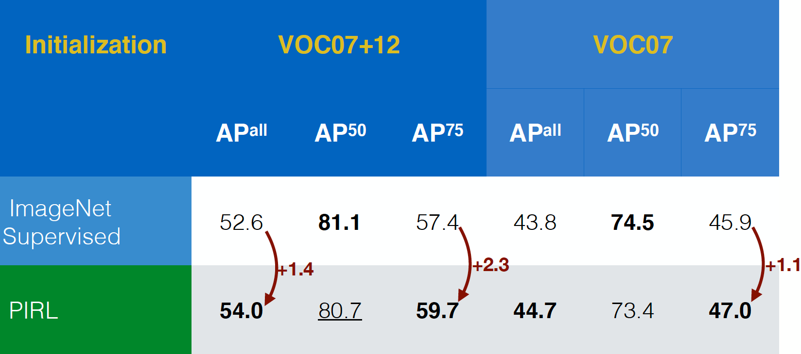
Fig. 17: Object detection performance on different datasets

Evaluating on Semi-supervised Learning

PIRL was then evaluated on semi-supervised learning task. Again, PIRL performed fairly well. In fact, PIRL was better than even the pre-text task of Jigsaw. The only difference between the first row and the last row is that, PIRL is an invariant version, whereas Jigsaw is a covariant version.

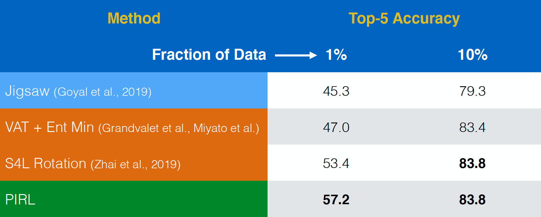
Fig. 18: Semi-supervised learning on ImageNet

Evaluating on Linear Classification

Now when evaluating on Linear Classifiers, PIRL was actually on par with the CPCv2, when it came out. It also worked well on a bunch of parameter settings and a bunch of different architectures. And of course, now you can have fairly good performance by methods like SimCLR or so. In fact, the Top-1 Accuracy for SimCLR would be around 69-70, whereas for PIRL, that’d be around 63.

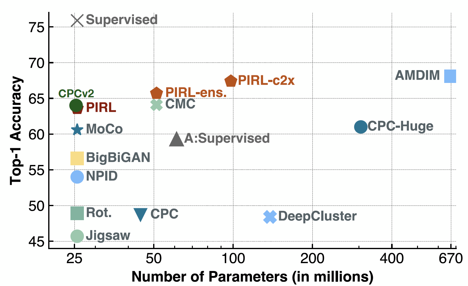
Fig. 19: ImageNet classification with linear models

Evaluating on YFCC images

PIRL was evaluated on “In-the-wild” Flickr images from the YFCC data set. It was able to perform better than Jigsaw, even with $100$ times smaller data set. This shows the power of taking invariance into consideration for the representation in the pre-text tasks, rather than just predicting pre-text tasks.

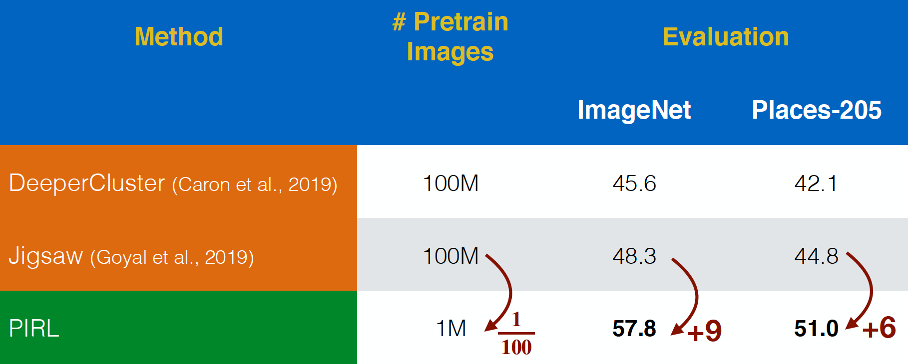
Fig. 20: Pre-training on uncurated YFCC images

Semantic Features

Now, going back to verifying the semantic features, we look at the Top-1 accuracy for PIRL and Jigsaw for different layers of representation from conv1 to res5. It’s interesting to note that the accuracy keeps increasing for different layers for both PIRL and Jigsaw, but drops in the 5th layer for Jigsaw. Whereas, the accuracy keeps improving for PIRL, i.e. more and more semantic.

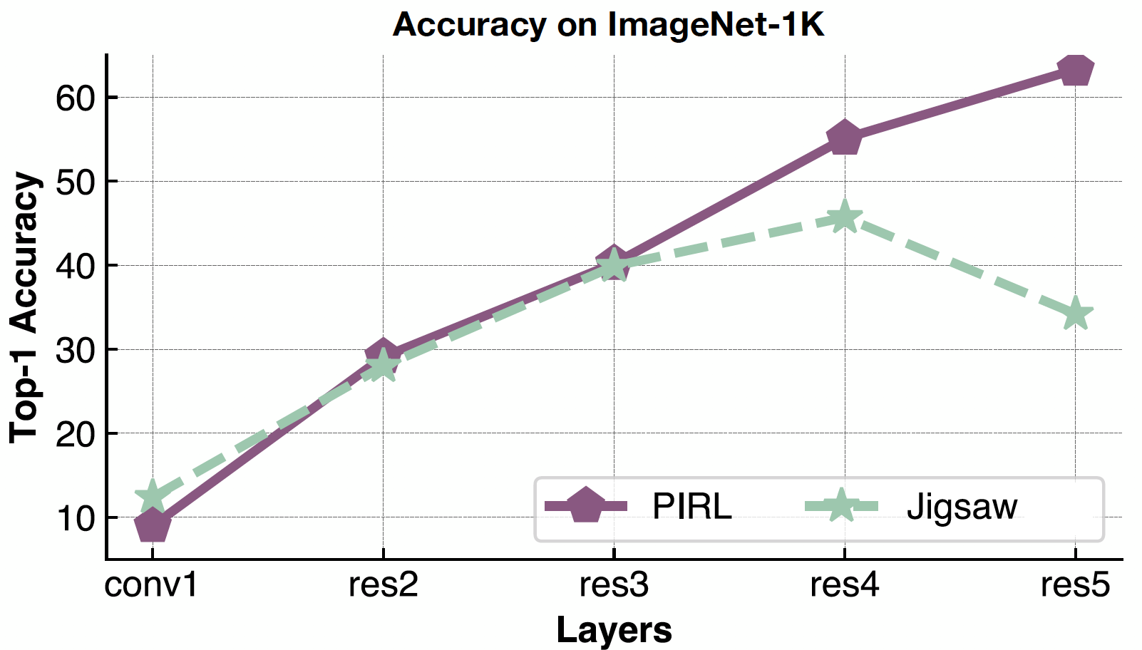
Fig. 21: Quality of PIRL representations per layer

Scalability

PIRL is very good at handling problem complexity because you’re never predicting the number of permutations, you’re just using them as input. So, PIRL can easily scale to all 362,880 possible permutations in the 9 patches. Whereas in Jigsaw, since you’re predicting that, you’re limited by the size of your output space.

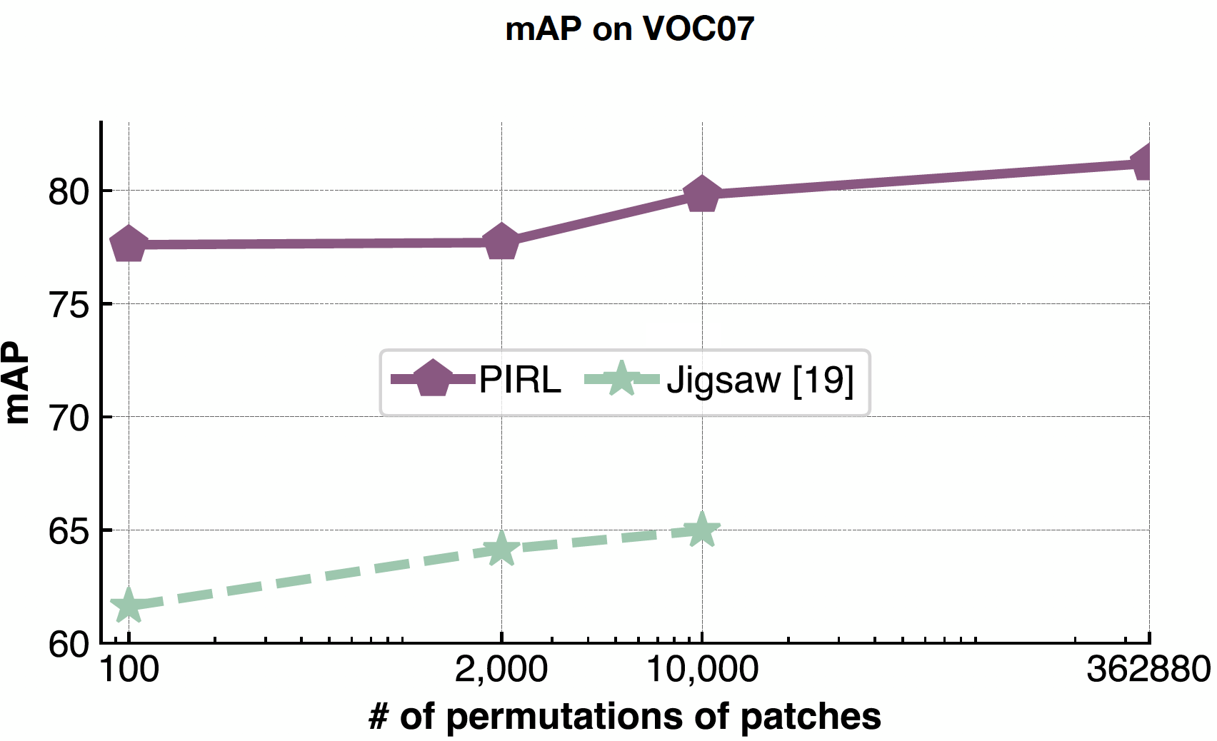
Fig. 22: Effect of varying the number of patch permutations

The paper “Misra & van der Maaten, 2019, PIRL” also shows how PIRL could be easily extended to other pretext tasks like Jigsaw, Rotations and so on. Further, it could even be extended to combinations of those tasks like Jigsaw+Rotation.

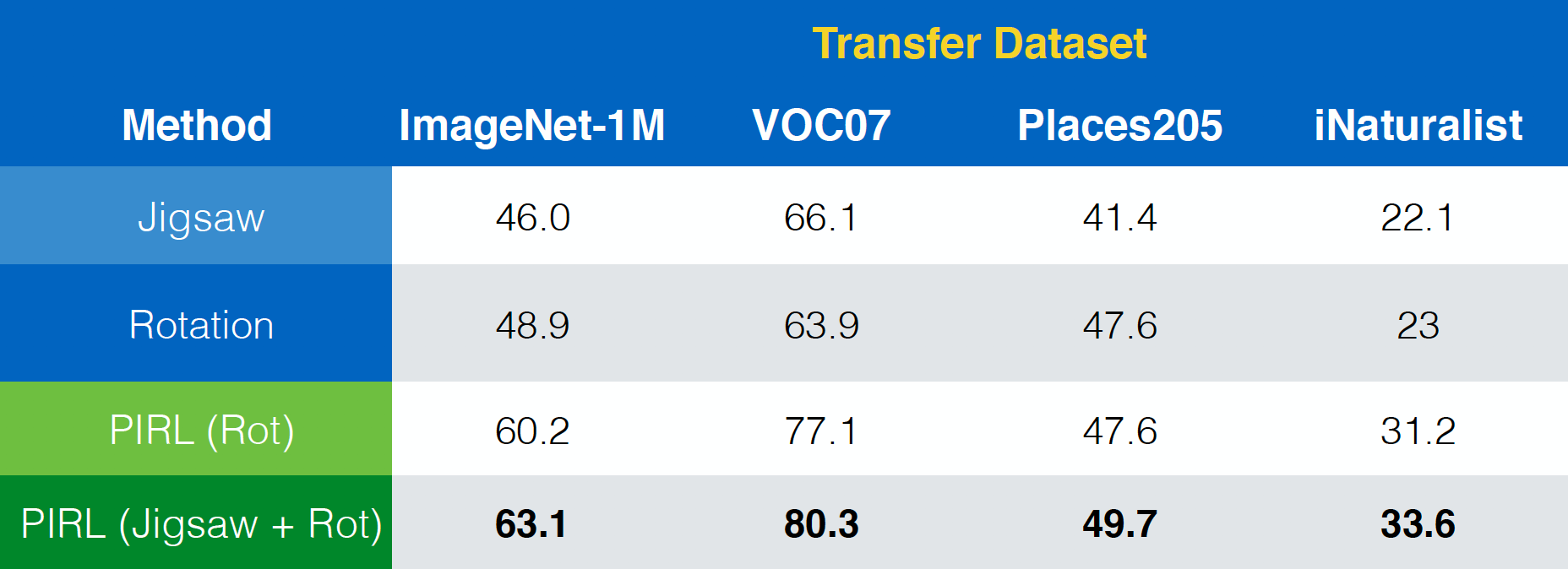
Fig. 23: Using PIRL with (combinations of) different pretext tasks

Invariance vs. performance

In terms of invariance property, one could, in general, assert that the invariance of PIRL is more than that of the Clustering, which in turn has more invariance than that of the pretext tasks. And similarly, the performance to is higher for PIRL than Clustering, which in turn has higher performance than pretext tasks. This suggests that taking more invariance in your method could improve performance.

Shortcomings

1. It’s not very clear as to which set of data transforms matter. Although Jigsaw works, it’s not very clear why it works.
2. Saturation with model size and data size.
3. What invariances matter? (One could think about what invariances work for a particular supervised task in general as future work.)

So in general, we should try to predict more and more information and try to be as invariant as possible.

Some important questions asked as doubts

Contrastive learning and batch norms

1. Wouldn’t the network learn only a very trivial way of separating the negatives from the positives if the contrasting network uses the batch norm layer (as the information would then pass from one sample to the other)?

Ans: In PIRL, no such phenomenon was observed, so just the usual batch norm was used

1. So is it fine to use batch norms for any contrasting networks?

Ans: In general, yeah. In SimCLR, a variant of the usual batch norm is used to emulate a large batch size. So, batch norm with maybe some tweaking could be used to make the training easier

1. Does the batch norm work in the PIRL paper only because it’s implemented as a memory bank - as all the representations aren’t taken at the same time? (As batch norms aren’t specifically used in the MoCo paper for instance)

Ans: Yeah. In PIRL, the same batch doesn’t have all the representations and possibly why batch norm works here, which might not be the case for other tasks where the representations are all correlated within the batch

1. So, other than memory bank, are there any other suggestions how to go about for n-pair loss? Should we use AlexNet or others that don’t use batch norm? Or is there a way to turn off the batch norm layer? (This is for a video learning task)

Ans: Generally frames are correlated in videos, and the performance of the batch norm degrades when there are correlations. Also, even the simplest implementation of AlexNet actually uses batch norm. Because, it’s much more stable when trained with a batch norm. You could even use a higher learning rate and you could also use for other downstream tasks. You could use a variant of batch norm for example, group norm for video learning task, as it doesn’t depend on the batch size

Loss functions in PIRL

1. In PIRL, why is NCE (Noise Contrastive Estimator) used for minimizing loss and not just the negative probability of the data distribution: $h(v_{I},v_{I^{t}})$?

Ans: Actually, both could be used. The reason for using NCE has more to do with how the memory bank paper was set up. So, with $k+1$ negatives, it’s equivalent to solving $k+1$ binary problem. Another way of doing it is using a softmax, where you apply a softmax and minimize the negative log-likelihood

Self-supervised learning project related tips

How do we get a simple self-supervised model working? How do we begin the implementation?

Ans: There are a certain class of techniques that are useful for the initial stages. For instance, you could look at the pretext tasks. Rotation is a very easy task to implement. The number of moving pieces are in general good indicator. If you’re planning to implement an existing method, then you might have to take a closer look at the details mentioned by the authors, like - the exact learning rate used, the way batch norms were used, etc. The more number of these things, the harder the implementation. Next very critical thing to consider is data augmentation. If you get something working, then add more data augmentation to it.

Generative models

Have you thought of combining generative models with contrasting networks?

Ans: Generally, it’s good idea. But, it hasn’t been implemented partly because it is tricky and non-trivial to train such models. Integrative approaches are harder to implement, but perhaps the way to go in the future.

Distillation

Wouldn’t the uncertainty of the model increase when richer targets are given by softer distributions? Also, why is it called distillation?

Ans: If you train on one hot labels, your models tend to be very overconfident. Tricks like label smoothing are being used in some methods. Label smoothing is just a simple version of distillation where you are trying to predict a one hot vector. Now, rather than trying to predict the entire one-hot vector, you take some probability mass out of that, where instead of predicting a one and a bunch of zeros, you predict say $0.97$ and then you add $0.01$, $0.01$ and $0.01$ to the remaining vector (uniformly). Distillation is just a more informed way of doing this. Instead of randomly increasing the probability of an unrelated task, you have a pre-trained network to do that. In general softer distributions are very useful in pre-training methods. Models tend to be over-confident and so softer distributions are easier to train. They converge faster too. These benefits are present in distillation