World Models and Generative Adversarial Networks

World models for autonomous control

One of the most important uses of self-supervised learning is to learn world models for control. When humans perform a task, we have an internal model for how the world works. For example, we gain an intuition for physics when we’re about 9 months old, mostly through observation. In some sense, this is similar to self-supervised learning; in learning to predict what will happen, we learn abstract principles, just like self-supervised models learn latent features. But taking this one step further, the internal models let us act on the world. For example, we can use our learned physics intuition and our learned understanding of how our muscles work to predict — and execute — how to catch a falling pen.

What is a “world model”?

An autonomous intelligence system comprises four major modules (Figure 1.). First, the perception module observes the world and computes a representation of the state of the world. This representation is incomplete because 1) the agent doesn’t observe the whole universe, and 2) the accuracy of the observations is limited. It is also worth noting that in the feed-forward model, the perception module is only present for the initial time step. Second, the actor module (also called a policy module) imagines taking some action based on the (represented) state of the world. Third, the model module predicts the outcome of the action given the (represented) state of the world, and also possibly given some latent features. This prediction gets passed forward to the next time step as the guess for the next state of the world, taking on the role of the perception module from the initial time step. Fig 2 gives an in-detail demonstration of this feed-forward process. Finally, the critic module turns that same prediction into a cost of performing the proposed action, e.g. given the speed with which I believe the pen is falling, if I move muscles in this particular way, how badly will I miss the catch?

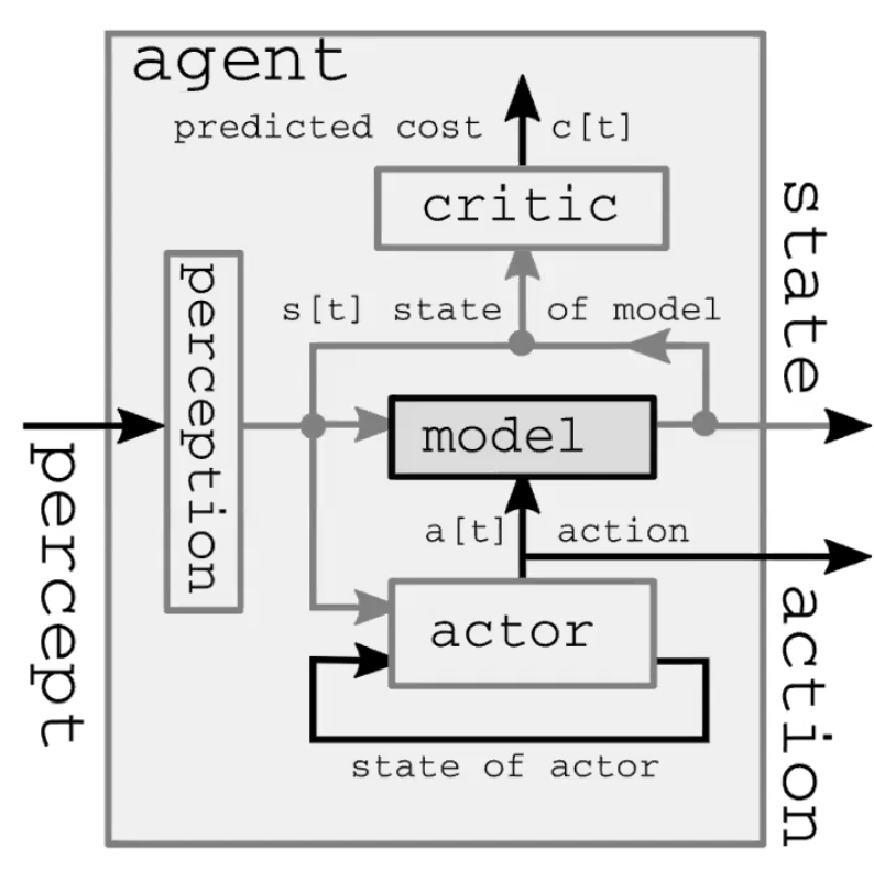
Fig. 1: The World Models architecture of an autonomous intelligence system demonstration.

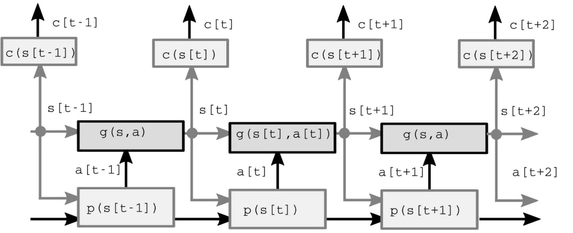
Fig. 2: Model architecture.

The classical setting

In classical optimal control, there is no actor/policy module, but rather just an action variable. This formulation is optimized by a classical method called Model Predictive Control, which was used by NASA in the 1960s to compute rocket trajectories when they switched from human computers (mostly Black women mathematicians) to electronic computers. We can think of this system as an unrolled RNN, and the actions as latent variables, and use backpropagation and gradient methods (or possibly other methods, such as dynamic programming for a discrete action set) to infer the sequence of actions that minimizes the sum of the time step costs.

Aside: We use the word “inference” for latent variables, and “learning” for parameters, though the process of optimizing them is generally similar. One important difference is that a latent variable takes a specific value for each sample, whereas, parameters are shared between samples.

An improvement

Now, we’d prefer not to go through the complicated process of backpropagating every time we want to make a plan. To address this, we use the same trick we used for variational autoencoder to improve sparse coding: we train an encoder to directly predict the optimal action sequence from the world representations. In this regime, the encoder is called a policy network.

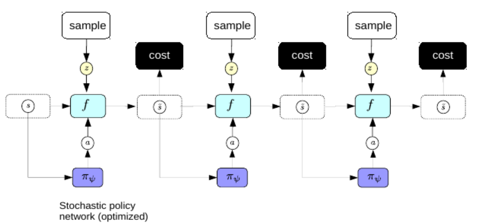
Fig. 3: Policy Network.

Once trained, we can use the policy networks to predict the optimal action sequence immediately after perception.

Reinforcement learning (RL)

The main differences between RL and what we have studied up to this point are two-fold:

1. In Reinforcement learning environments, the cost function is a black box. In other words, the agent does not understand the reward dynamics.
2. In the setting of RL, we don’t use a forward model of the world to step the environment. Instead we interact with the real world and learn the result by observing what happens. In the real world our measure of the state of the world is imperfect so it is not always possible to predict what will happen next.

The main problem of Reinforcement learning is that the cost function is not differentiable. This means that the only way to learn is through trial and error. Then the problem becomes how to explore the state space efficiently. Once you come up with a solution to this the next issue is the fundamental question of exploration vs. exploitation: would you rather take actions to maximally learn about the environment or instead exploit what you have already learned to get as high a reward as possible?

Actor-Critic methods are a popular family of RL algorithms which train both an actor and a critic. Many RL methods work similarly, by training a model of the cost function (the critic). In Actor-Critic methods the role of the critic is to learn the expected value of the value function. This enables back-propagation through the module, since the critic is just a neural network. The actor’s responsibility is to propose actions to take in the environment, and the critic’s job is to learn a model of the cost function. The actor and the critic work in tandem that leads to more efficient learning than if no critic is used. If you don’t have a good model of the world it is much more difficult to learn: e.g. the car next to the cliff will not know that falling off a cliff is a bad idea. This enables humans and animals to learn much more quickly than RL agents: we have really good world models in our head.

We cannot always predict the future of the world due to inherent uncertainty: aleatory and epistemic uncertainty. Aleatoric uncertainty is due to things you cannot control or observe in the environment. Epistemic uncertainty is when you cannot predict the future of the world because your model does not have enough training data.

The forward model would like to be able to predict

where $z$ is a latent variable of which we don’t know the value. $z$ represents what you cannot know about the world but which still influences the prediction (i.e. aleatoric uncertainty). We can regularize $z$ with sparsity, noise, or with an encoder. We can use forward models to learn to plan. The system works by having a decoder decode a concatenation of the state representation and the uncertainty $z$. The best $z$ is defined as the $z$ that minimizes the difference between $\hat s_{t+1}$ and the actual observed $s_{t+1}$.

Generative Adversarial Network

There are many variations of GAN and here we think of GAN as a form of energy-based model using contrastive methods. It pushes up the energy of contrastive samples and pushes down the energy of training samples. A basic GAN consists of two parts: a generator which produces contrastive samples intelligently and a discriminator (sometimes called critic) which is essentially a cost function and acts as an energy model. Both the generator and the discriminator are neural nets.

The two kinds of input to GAN are respectively training samples and contrastive samples. For training samples, GAN passes these samples through the discriminator and makes their energy go down. For contrastive samples, GAN samples latent variables from some distribution, runs them through the generator to produce something similar to training samples, and passes them through the discriminator to make their energy go up. The loss function for discriminator is as follows:

where $L_d$ can be a margin-based loss function like $F(y) + [m - F(\bar{y})]^+$ or $\log(1 + \exp[F(y)]) + \log(1 + \exp[-F(\bar{y})])$ as long as it makes $F(y)$ decrease and $F(\bar{y})$ increase. In this context, $y$ is the label, and $\bar{y}$ is the response variable gives lowest energy except $y$ itself. There is going to be a different loss function for the generator:

where $z$ is the latent variable and $G$ is the generator neural net. We want to make the generator adapt its weight and produce $\bar{y}$ with low energy that can fool the discriminator.

The reason why this type of model is called generative adversarial network is because we have two objective functions that are incompatible with each other and we need to minimize them simultaneously. It’s not a gradient descent problem because the goal is to find a Nash equilibrium between these two functions and gradient descent is not capable of this by default.

There will be problems when we have samples that are close to the true manifold. Assume that we have an infinitely thin manifold. The discriminator needs to produce $0$ probability outside the manifold and infinite probability on the manifold. Since this is very difficult to achieve, GAN uses sigmoid and produces $0$ outside the manifold and produces $1$ on the manifold. The problem with this is that if we train the system successfully where we get the discriminator to produce $0$ outside the manifold, the energy function is completely useless. This is because the energy function is not smooth where all energy outside the data manifold will be infinity and all energy on the data manifold will be $0$. We don’t want the energy value to go from $0$ to infinity in a very small step. Researchers have proposed many ways to fix this problem by regularizing the energy function. A good example of improved GAN is Wasserstein GAN which limits the size of discriminator weight.