Regularized Latent Variable Energy Based Models

Regularized latent variable EBMs

Models with latent variables are capable of making a distribution of predictions $\overline{y}$ conditioned on an observed input $x$ and an additional latent variable $z$. Energy-based models can also contain latent variables:

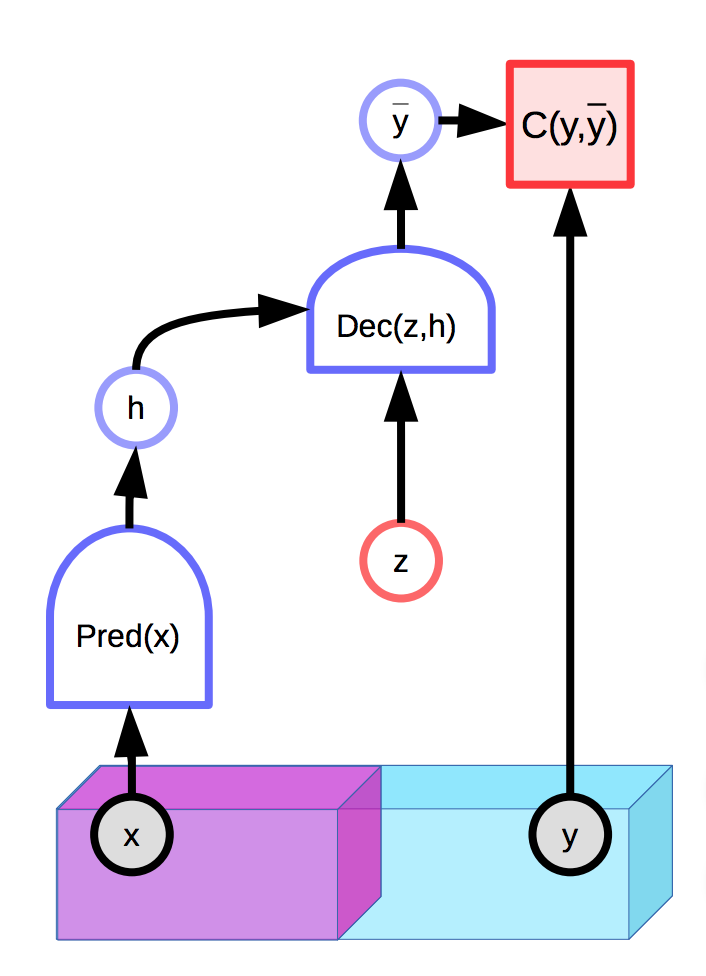
Fig. 1: Example of an EBM with a latent variable

See the previous lecture’s notes for more details.

Unfortunately, if the latent variable $z$ has too much expressive power in producing the final prediction $\overline{y}$, every true output $y$ will be perfectly reconstructed from input $x$ with an appropriately chosen $z$. This means that the energy function will be 0 everywhere, since the energy is optimized over both $y$ and $z$ during inference.

A natural solution is to limit the information capacity of the latent variable $z$. One way to do this is to regularize the latent variable:

This method will limit the volume of space of $z$ which takes a small value and the value which will, in turn, controls the space of $y$ that has low energy. The value of $\lambda$ controls this tradeoff. A useful example of $R$ is the $L_1$ norm, which can be viewed as an almost everywhere differentiable approximation of effective dimension. Adding noise to $z$ while limiting its $L_2$ norm can also limit its information content (VAE).

Sparse Coding

Sparse coding is an example of an unconditional regularized latent-variable EBM which essentially attempts to approximate the data with a piecewise linear function.

The $n$-dimensional vector $z$ will tend to have a maximum number of non-zero components $m « n$. Then each $Wz$ will be elements in the span of $m$ columns of $W$.

After each optimization step, the matrix $W$ and latent variable $z$ are normalized by the sum of the $L_2$ norms of the columns of $W$. This ensures that $W$ and $z$ do not diverge to infinity and zero.

FISTA

Fig. 2: FISTA computation graph

FISTA (fast ISTA) is an algorithm that optimizes the sparse coding energy function $E(y,z)$ with respect to $z$ by alternately optimizing the two terms $\Vert y - Wz\Vert^2$ and $\lambda \Vert z\Vert_{L^1}$. We initialize $Z(0)$ and iteratively update $Z$ according to the following rule:

The inner expression $Z(t) - \frac{1}{L}W_d^\top(W_dZ(t) - Y)$ is a gradient step for the $\Vert y - Wz\Vert^2$ term. The $\text{Shrinkage}$ function then shifts values towards 0, which optimizes the $\lambda \Vert z\Vert_{L_1}$ term.

LISTA

FISTA is too expensive to apply to large sets of high-dimensional data (e.g. images). One way to make it more efficient is to instead train a network to predict the optimal latent variable $z$:

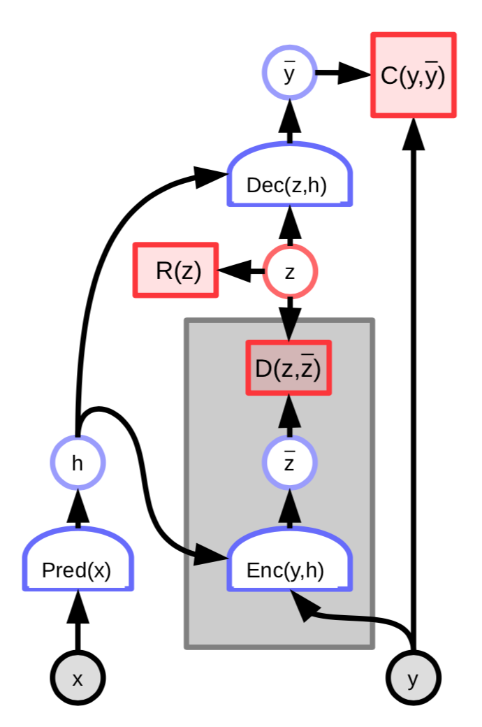
Fig. 3: EBM with latent variable encoder

The energy of this architecture then includes an additional term that measures the difference between the predicted latent variable $\overline z$ and the optimal latent variable $z$:

We can further define

and then write

This update rule can be interpreted as a recurrent network, which suggests that we can instead learn the parameters $W_e$ that iteratively determine the latent variable $z$. The network is run for a fixed number of time steps $K$ and the gradients of $W_e$ are computed using standard backpropagation-through-time. The trained network then produces a good $z$ in fewer iterations than the FISTA algorithm.

Fig. 4: LISTA as a recurrent net unfolded through time.

Sparse coding examples

When a sparse coding system with 256 dimensional latent vector is applied to MNIST handwritten digits, the system learns a set of 256 strokes that can be linearly combined to nearly reproduce the entire training set. The sparse regularizer ensures that they can be reproduced from a small number of strokes.

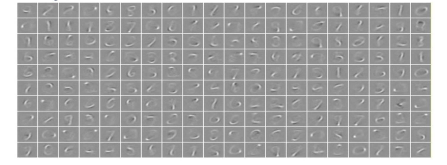
Fig. 5: Sparse coding on MNIST. Each image is a learned column of $W$.

When a sparse coding system is trained on natural image patches, the learned features are Gabor filters, which are oriented edges. These features resemble features learned in early parts of animal visual systems.

Convolutional sparse coding

Suppose, we have an image and the feature maps ($z_1, z_2, \cdots, z_n$) of the image. Then we can convolve ($*$) each of the feature maps with the kernel $K_i$. Then the reconstruction can be simply calculated as:

This is different from the original sparse coding where the reconstruction was done as $Y=\sum_{i}W_iZ_i$. In regular sparse coding, we have a weighted sum of columns where the weights are coefficients of $Z_i$. In convolutional sparse coding, it is still a linear operation but the dictionary matrix is now a bunch of feature maps and we convolve each feature map with each kernel and sum up the results.

Convolutional sparse auto-encoder on natural images

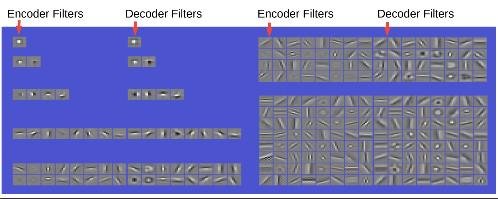
Fig.6 Filters and Basis Functions obtained. Linear convolutional decoder

The filters in the encoder and decoder look very similar. Encoder is simply a convolution followed by some non-linearity and then a diagonal layer to change the scale. Then there is sparsity on the constraint of the code. The decoder is just a convolutional linear decoder and the reconstruction here is the square error.

So, if we impose that there is only one filter then it is just a centre surround type filter. With two filters, we can get some weird shaped filters. With four filters, we get oriented edges (horizontal and vertical); we get 2 polarities for each of the filters. With eight filters we can get oriented edges at 8 different orientations. With 16, we get more orientation along with the centres around. As we go on increasing the filters, we get more diverse filters that is in addition to edge detectors, we also get grating detectors of various orientations, centres around, etc.

This phenomenon seems to be interesting since it is similar to what we observe in the visual cortex. So this is an indication that we can learn really good features in a completely unsupervised way.

As a side use, if we take these features and plug them in a convolutional net and then train them on some task, then we don’t necessarily get better results than training an image net from scratch. However, there are some instances where it can help to boost performance. For instance, in cases where the number of samples are not large enough or there are few categories, by training in a purely supervised manner, we get degenerate features.

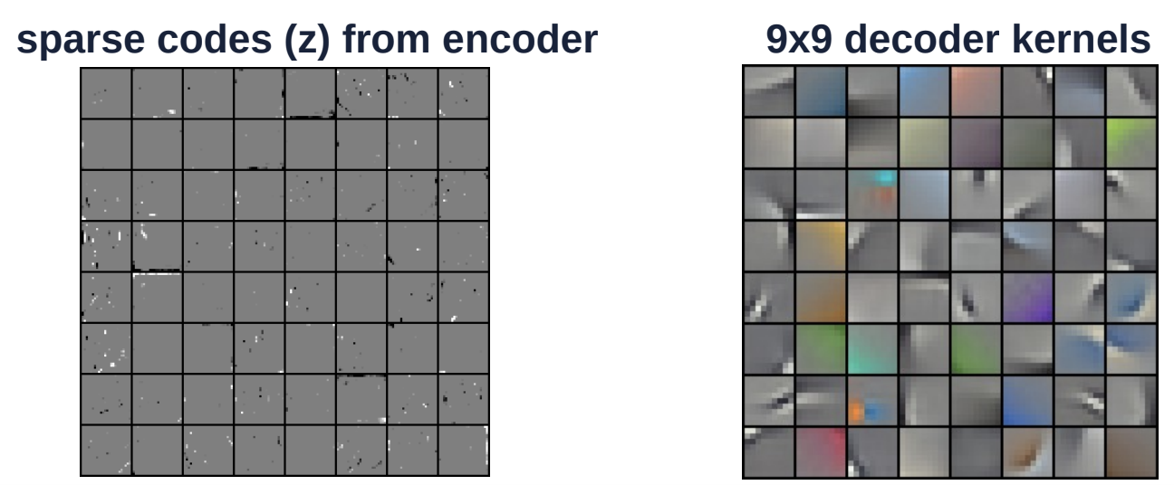
Fig. 7 Convolutional sparse encoding on colour image

The figure above is another example on colour images. The decoding kernel (on the right side) is of size 9 by 9. This kernel is applied convolutionally over the entire image. The image on the left is of the sparse codes from the encoder. The $Z$ vector is very sparse space where there are just few components that are white or black (non-grey).

Variational autoencoder

Variational Autoencoders have an architecture similar to Regularized Latent Variable EBM, with the exception of sparsity. Instead, the information content of the code is limited by making it noisy.

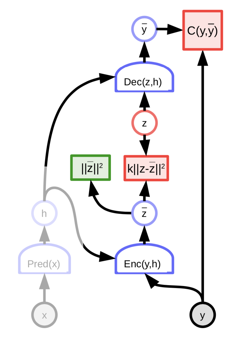
Fig. 8: Architecture of Variational Autoencoder

The latent variable $z$ is not computed by minimizing the energy function with respect to $z$. Instead, the energy function is viewed as sampling $z$ randomly according to a distribution whose logarithm is the cost that links it to ${\overline z}$. The distribution is a Gaussian with mean ${\overline z}$ and this results in Gaussian noise being added to ${\overline z}$.

The code vectors with added Gaussian noise can be visualized as fuzzy balls as shown in Fig. 9(a).

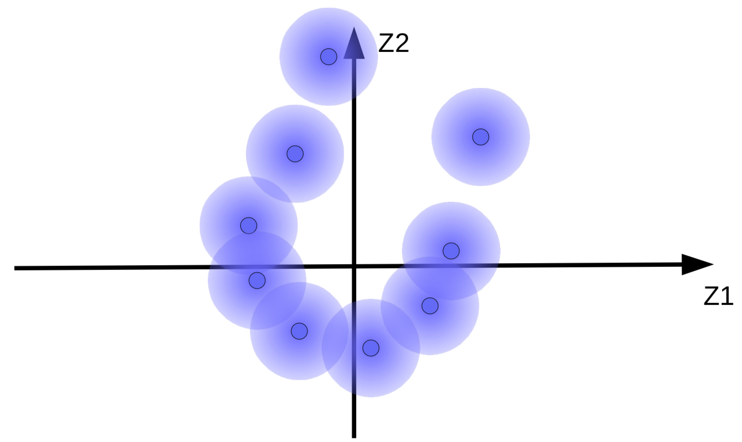(a) Original set of fuzzy balls

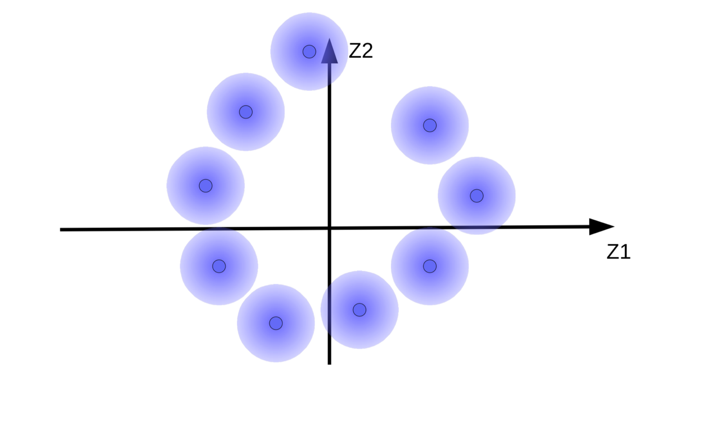(b) Movement of fuzzy balls due to energy minimization without regularization

The system tries to make the code vectors ${\overline z}$ as large as possible so that the effect of $z$(noise) is as small as possible. This results in the fuzzy balls floating away from the origin as shown in Fig. 9(b). Another reason why the system tries to make the code vectors large is to prevent overlapping fuzzy balls, which causes the decoder to confuse between different samples during reconstruction.

But we want the fuzzy balls to cluster around a data manifold, if there is one. So, the code vectors are regularized to have a mean and variance close to zero. To do this, we link them to the origin by a spring as shown in Fig. 10.

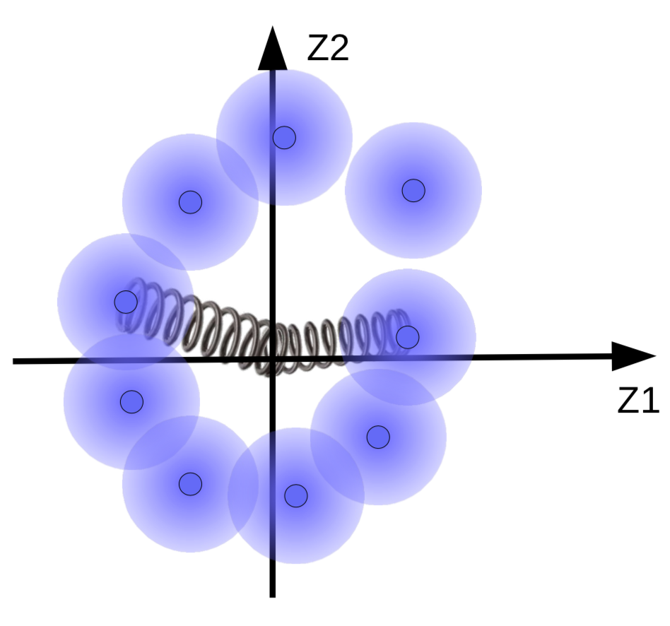
Fig. 10: Effects of regularization visualized with springs

The strength of the spring determines how close the fuzzy balls are to the origin. If the spring is too weak, then the fuzzy balls would fly away from the origin. And if it’s too strong, then they would collapse at the origin, resulting in a high energy value. To prevent this, the system lets the spheres overlap only if the corresponding samples are similar.

It is also possible to adapt the size of the fuzzy balls. This is limited by a penalty function (KL Divergence) that tries to make the variance close to 1 so that the size of the ball is neither too big nor too small that it collapses.