Introduction to autoencoders

Application of autoencoders

Image generation

Can you tell which face is fake in Fig. 1? In fact, both of them are produced by the StyleGan2 generator. Although the facial details are very realistic, the background looks weird (left: blurriness, right: misshapen objects). This is because the neural network is trained on faces samples. The background then has a much higher variability. Here the data manifold has roughly 50 dimensions, equal to the degrees of freedom of a face image.

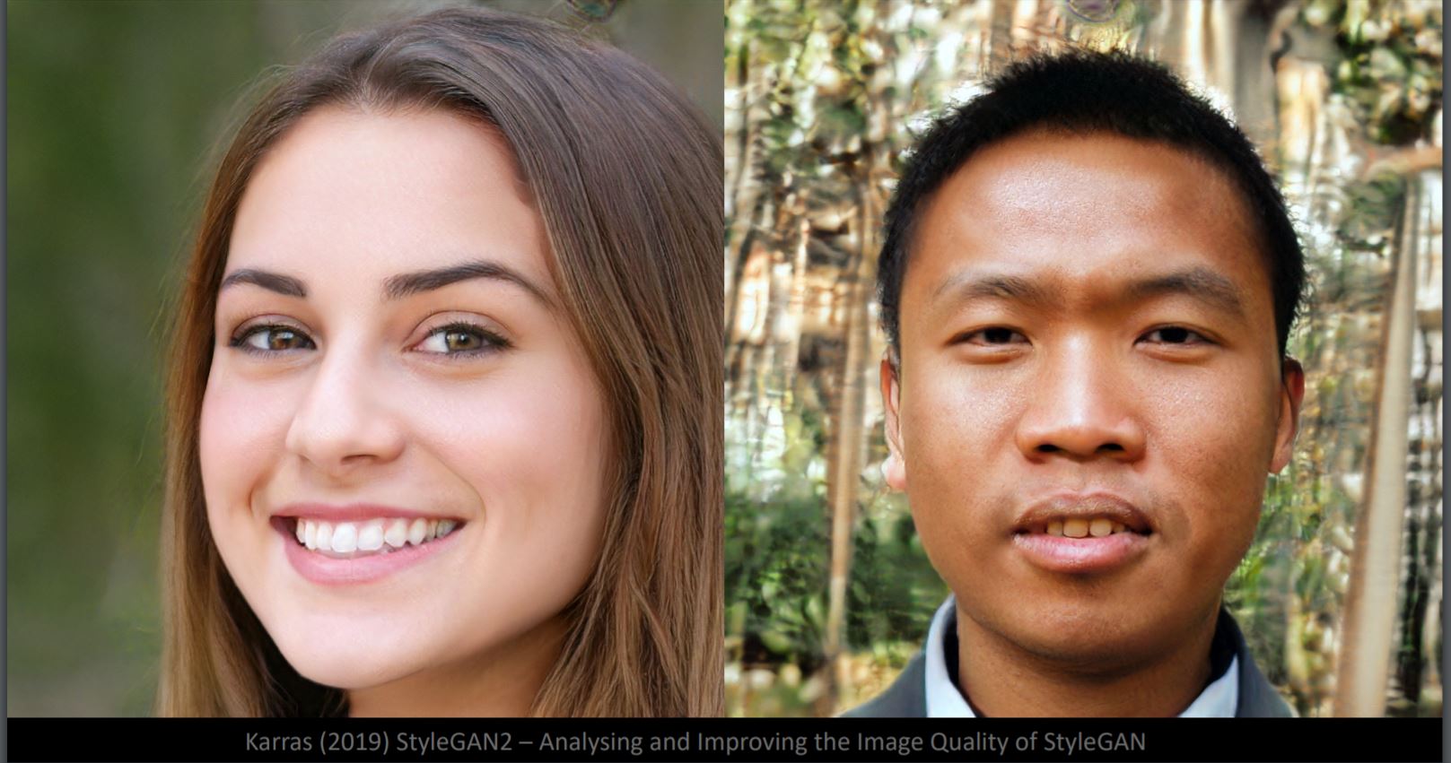
Fig. 1: Faces generated from StyleGan2

Difference of Interpolation in Pixel Space and Latent Space

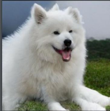
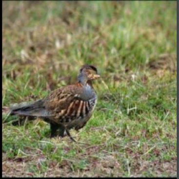
Fig. 2: A dog and a bird

If we linearly interpolate between the dog and bird image (Fig. 2) in pixel space, we will get a fading overlay of two images in Fig. 3. From the top left to the bottom right, the weight of the dog image decreases and the weight of the bird image increases.

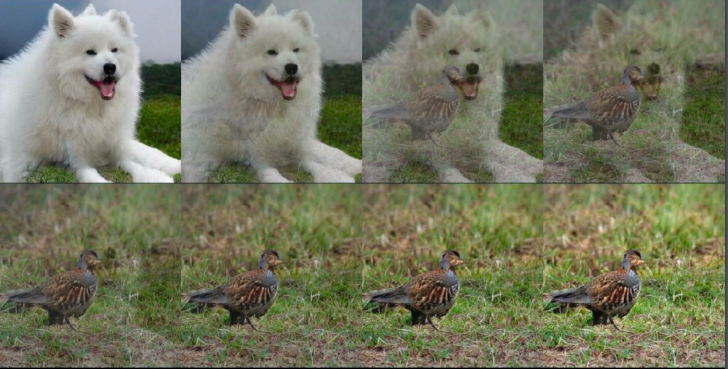
Fig. 3: Results after interpolation

If we interpolate on two latent space representation and feed them to the decoder, we will get the transformation from dog to bird in Fig. 4.

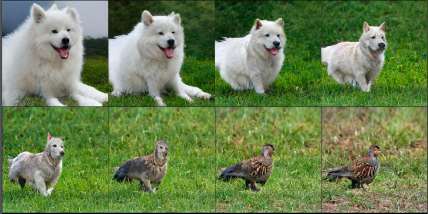
Fig. 4: Results after feeding into decoder

Obviously, latent space is better at capturing the structure of an image.

Transformation Examples

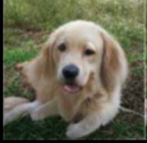
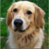
Fig. 5: Zoom

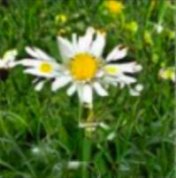
Fig. 6: Shift

Fig. 7: Brightness

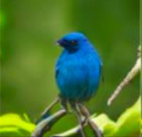
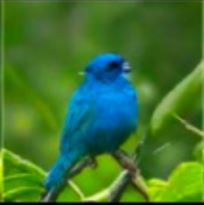
Fig. 8: Rotation (Note that the rotation could be 3D)

Image Super-resolution

This model aims to upscale images and reconstruct the original faces. From left to right in Fig. 9, the first column is the 16x16 input image, the second one is what you would get from a standard bicubic interpolation, the third is the output generated by the neural net, and on the right is the ground truth. (https://github.com/david-gpu/srez)

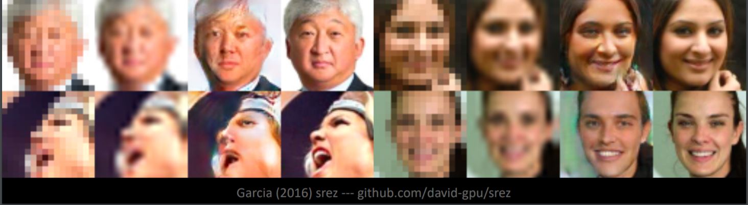
Fig. 9: Reconstructing original faces

From the output images, it is clear that there exist biases in the training data, which makes the reconstructed faces inaccurate. For example, the top left Asian man is made to look European in the output due to the imbalanced training images. The reconstructed face of the bottom left women looks weird due to the lack of images from that odd angle in the training data.

Image Inpainting

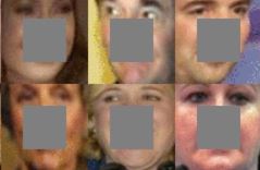
Fig. 10: Putting grey patch on faces

Putting a grey patch on the face like in Fig. 10 makes the image away from the training manifold. The face reconstruction in Fig. 11 is done by finding the closest sample image on the training manifold via Energy function minimization.

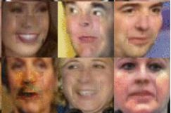
Fig. 11: Reconstructed image of Fig. 10

Caption to Image

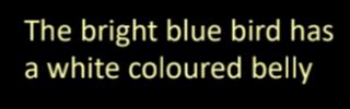
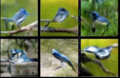
Fig. 12: Caption to Image example

The translation from text description to image in Fig. 12 is achieved by extracting text features representations associated with important visual information and then decoding them to images.

What are autoencoders?

Autoencoders are artificial neural networks, trained in an unsupervised manner, that aim to first learn encoded representations of our data and then generate the input data (as closely as possible) from the learned encoded representations. Thus, the output of an autoencoder is its prediction for the input.

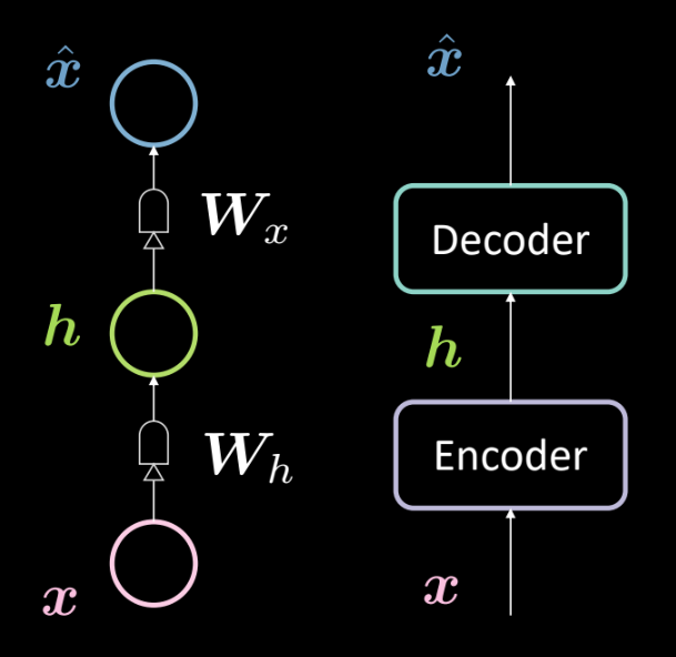
Fig. 13: Architecture of a basic autoencoder

Fig. 13 shows the architecture of a basic autoencoder. As before, we start from the bottom with the input $\boldsymbol{x}$ which is subjected to an encoder (affine transformation defined by $\boldsymbol{W_h}$, followed by squashing). This results in the intermediate hidden layer $\boldsymbol{h}$. This is subjected to the decoder(another affine transformation defined by $\boldsymbol{W_x}$ followed by another squashing). This produces the output $\boldsymbol{\hat{x}}$, which is our model’s prediction/reconstruction of the input. As per our convention, we say that this is a 3 layer neural network.

We can represent the above network mathematically by using the following equations:

We also specify the following dimensionalities:

Note: In order to represent PCA, we can have tight weights (or tied weights) defined by $\boldsymbol{W_x}\ \dot{=}\ \boldsymbol{W_h}^\top$

Why are we using autoencoders?

At this point, you may wonder what the point of predicting the input is and what are the applications of autoencoders.

The primary applications of an autoencoder is for anomaly detection or image denoising. We know that an autoencoder’s task is to be able to reconstruct data that lives on the manifold i.e. given a data manifold, we would want our autoencoder to be able to reconstruct only the input that exists in that manifold. Thus we constrain the model to reconstruct things that have been observed during training, and so any variation present in new inputs will be removed because the model would be insensitive to those kinds of perturbations.

Another application of an autoencoder is as an image compressor. If we have an intermediate dimensionality $d$ lower than the input dimensionality $n$, then the encoder can be used as a compressor and the hidden representations (coded representations) would address all (or most) of the information in the specific input but take less space.

Reconstruction loss

Let us now look at the reconstruction losses that we generally use. The overall loss for the dataset is given as the average per sample loss i.e.

When the input is categorical, we could use the Cross-Entropy loss to calculate the per sample loss which is given by

And when the input is real-valued, we may want to use the Mean Squared Error Loss given by

Under-/over-complete hidden layer

When the dimensionality of the hidden layer $d$ is less than the dimensionality of the input $n$ then we say it is under complete hidden layer. And similarly, when $d>n$, we call it an over-complete hidden layer. Fig. 14 shows an under-complete hidden layer on the left and an over-complete hidden layer on the right.

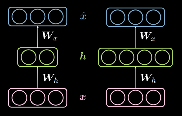
Fig. 14: An under-complete *vs.* an over-complete hidden layer

As discussed above, an under-complete hidden layer can be used for compression as we are encoding the information from input in fewer dimensions. On the other hand, in an over-complete layer, we use an encoding with higher dimensionality than the input. This makes optimization easier.

Since we are trying to reconstruct the input, the model is prone to copying all the input features into the hidden layer and passing it as the output thus essentially behaving as an identity function. This needs to be avoided as this would imply that our model fails to learn anything. Hence, we need to apply some additional constraints by applying an information bottleneck. We do this by constraining the possible configurations that the hidden layer can take to only those configurations seen during training. This allows for a selective reconstruction (limited to a subset of the input space) and makes the model insensitive to everything not in the manifold.

It is to be noted that an under-complete layer cannot behave as an identity function simply because the hidden layer doesn’t have enough dimensions to copy the input. Thus an under-complete hidden layer is less likely to overfit as compared to an over-complete hidden layer but it could still overfit. For example, given a powerful encoder and a decoder, the model could simply associate one number to each data point and learn the mapping. There are several methods to avoid overfitting such as regularization methods, architectural methods, etc.

Denoising autoencoder

Fig.15 shows the manifold of the denoising autoencoder and the intuition of how it works.

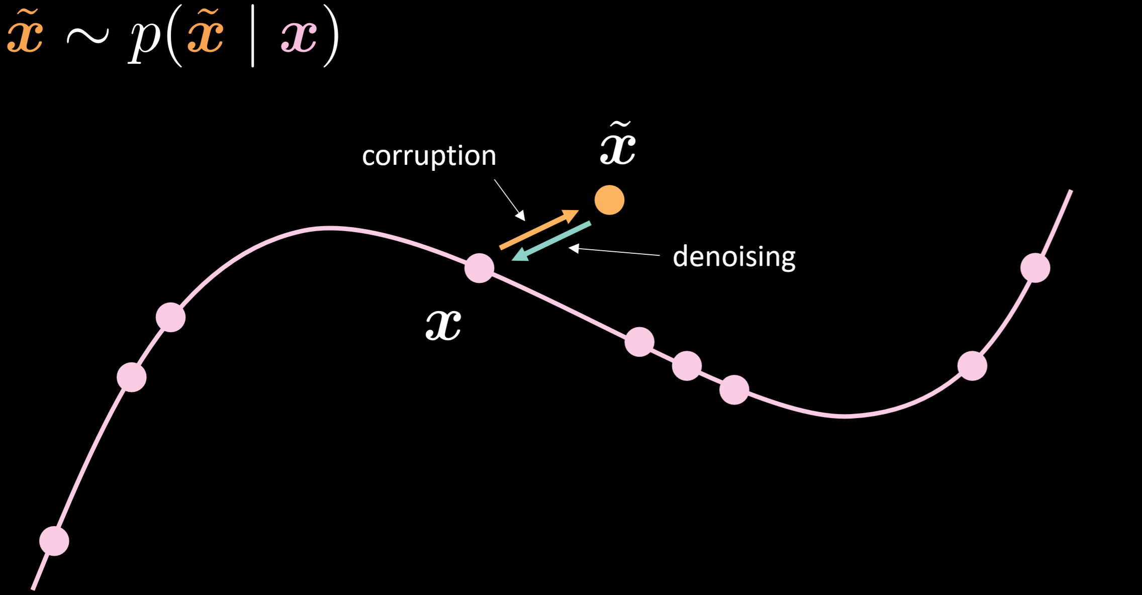
Fig. 15: Denoising autoencoder

In this model, we assume we are injecting the same noisy distribution we are going to observe in reality, so that we can learn how to robustly recover from it. By comparing the input and output, we can tell that the points that already on the manifold data did not move, and the points that far away from the manifold moved a lot.

Fig.16 gives the relationship between the input data and output data.

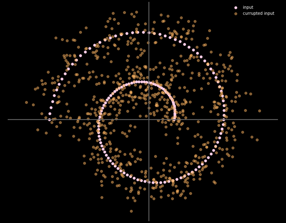
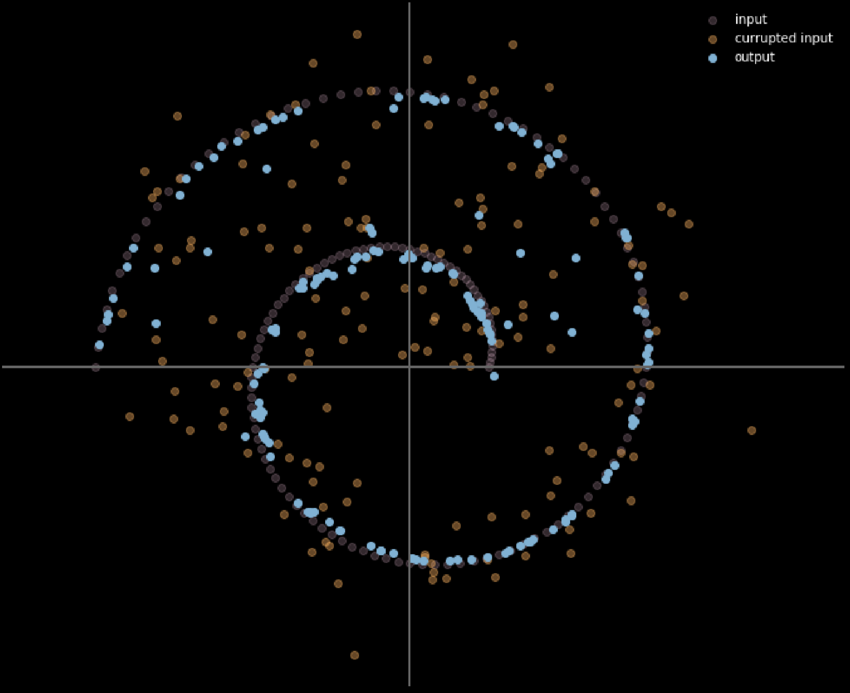
Fig. 16: Input and output of denoising autoencoder

We can also use different colours to represent the distance of each input point moves, Fig.17 shows the diagram.

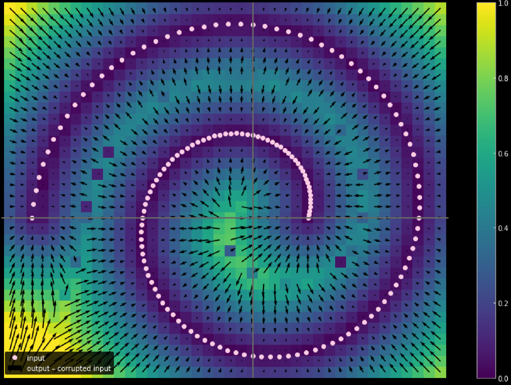
Fig. 17: Measuring the traveling distance of the input data

The lighter the colour, the longer the distance a point travelled. From the diagram, we can tell that the points at the corners travelled close to 1 unit, whereas the points within the 2 branches didn’t move at all since they are attracted by the top and bottom branches during the training process.

Contractive autoencoder

Fig.18 shows the loss function of the contractive autoencoder and the manifold.

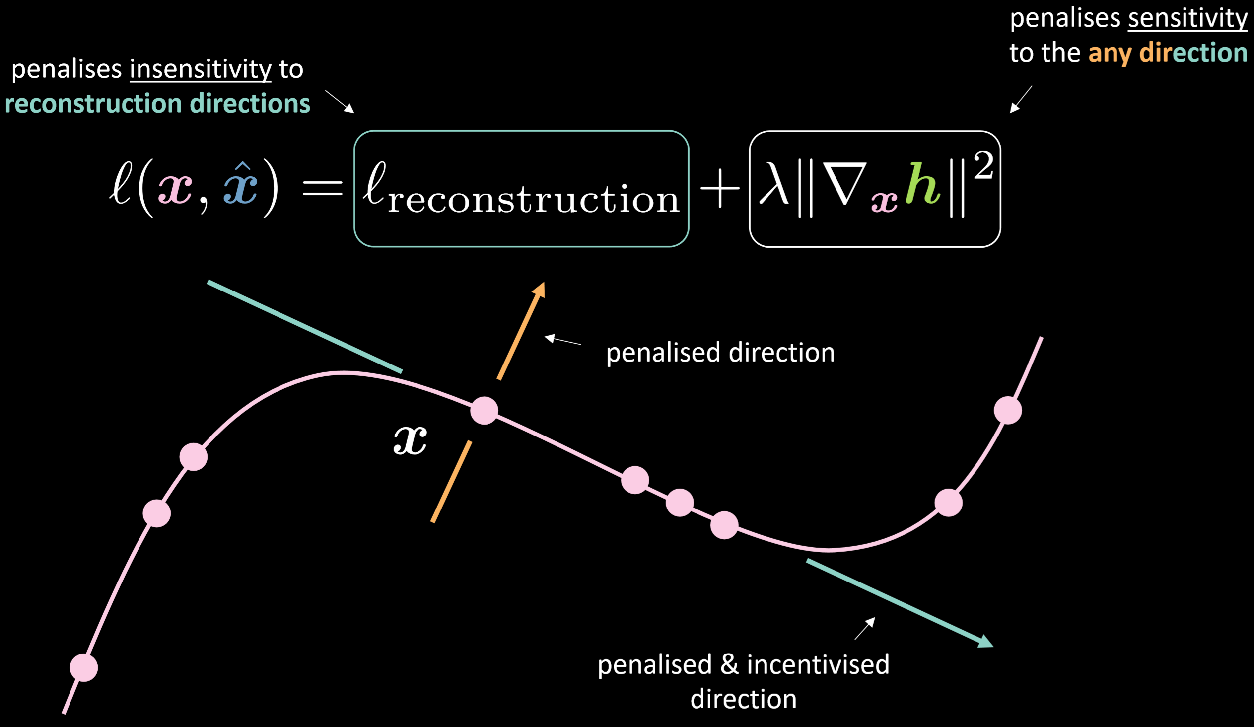
Fig. 18: Contractive autoencoder

The loss function contains the reconstruction term plus squared norm of the gradient of the hidden representation with respect to the input. Therefore, the overall loss will minimize the variation of the hidden layer given variation of the input. The benefit would be to make the model sensitive to reconstruction directions while insensitive to any other possible directions.

Fig.19 shows how these autoencoders work in general.

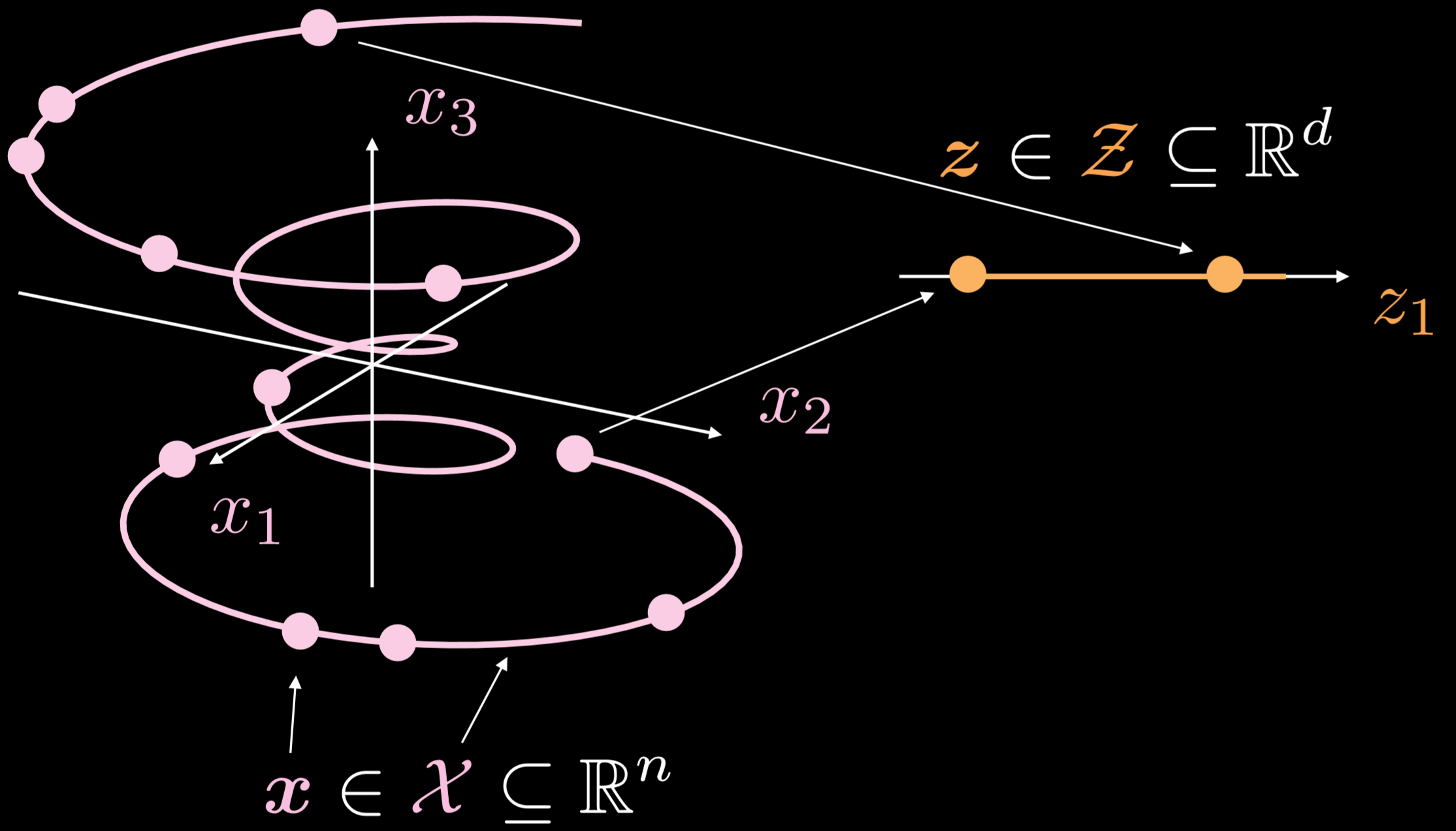
Fig. 19: Basic autoencoder

The training manifold is a single-dimensional object going in three dimensions. Where $\boldsymbol{x}\in \boldsymbol{X}\subseteq\mathbb{R}^{n}$, the goal for autoencoder is to stretch down the curly line in one direction, where $\boldsymbol{z}\in \boldsymbol{Z}\subseteq\mathbb{R}^{d}$. As a result, a point from the input layer will be transformed to a point in the latent layer. Now we have the correspondence between points in the input space and the points on the latent space but do not have the correspondence between regions of the input space and regions of the latent space. Afterwards, we will utilize the decoder to transform a point from the latent layer to generate a meaningful output layer.

Implement autoencoder - Notebook

The Jupyter Notebook can be found here.

In this notebook, we are going to implement a standard autoencoder and a denoising autoencoder and then compare the outputs.

Define autoencoder model architecture and reconstruction loss

Using $28 \times 28$ image, and a 30-dimensional hidden layer. The transformation routine would be going from $784\to30\to784$. By applying hyperbolic tangent function to encoder and decoder routine, we are able to limit the output range to $(-1, 1)$. Mean Squared Error (MSE) loss will be used as the loss function of this model.

class Autoencoder(nn.Module):
    def __init__(self):
        super().__init__()
        self.encoder = nn.Sequential(
            nn.Linear(n, d),
            nn.Tanh(),
        )
        self.decoder = nn.Sequential(
            nn.Linear(d, n),
            nn.Tanh(),
        )

    def forward(self, x):
        x = self.encoder(x)
        x = self.decoder(x)
        return x

model = Autoencoder().to(device)
criterion = nn.MSELoss()

Train standard autoencoder

To train a standard autoencoder using PyTorch, you need put the following 5 methods in the training loop:

Going forward:

1) Sending the input image through the model by calling output = model(img) .
2) Compute the loss using: criterion(output, img.data).

Going backward:

3) Clear the gradient to make sure we do not accumulate the value: optimizer.zero_grad().
4) Back propagation: loss.backward()
5) Step backwards: optimizer.step()

Fig. 20 shows the output of the standard autoencoder.

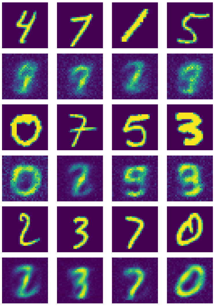
Fig. 20: Output of standard autoencoder

Train denoising autoencoder

For denoising autoencoder, you need to add the following steps:
1) Calling do = nn.Dropout() creates a function that randomly turns off neurons.
2) Create noise mask: do(torch.ones(img.shape)).
3) Create bad images by multiply good images to the binary masks: img_bad = (img * noise).to(device).

Fig. 21 shows the output of the denoising autoencoder.

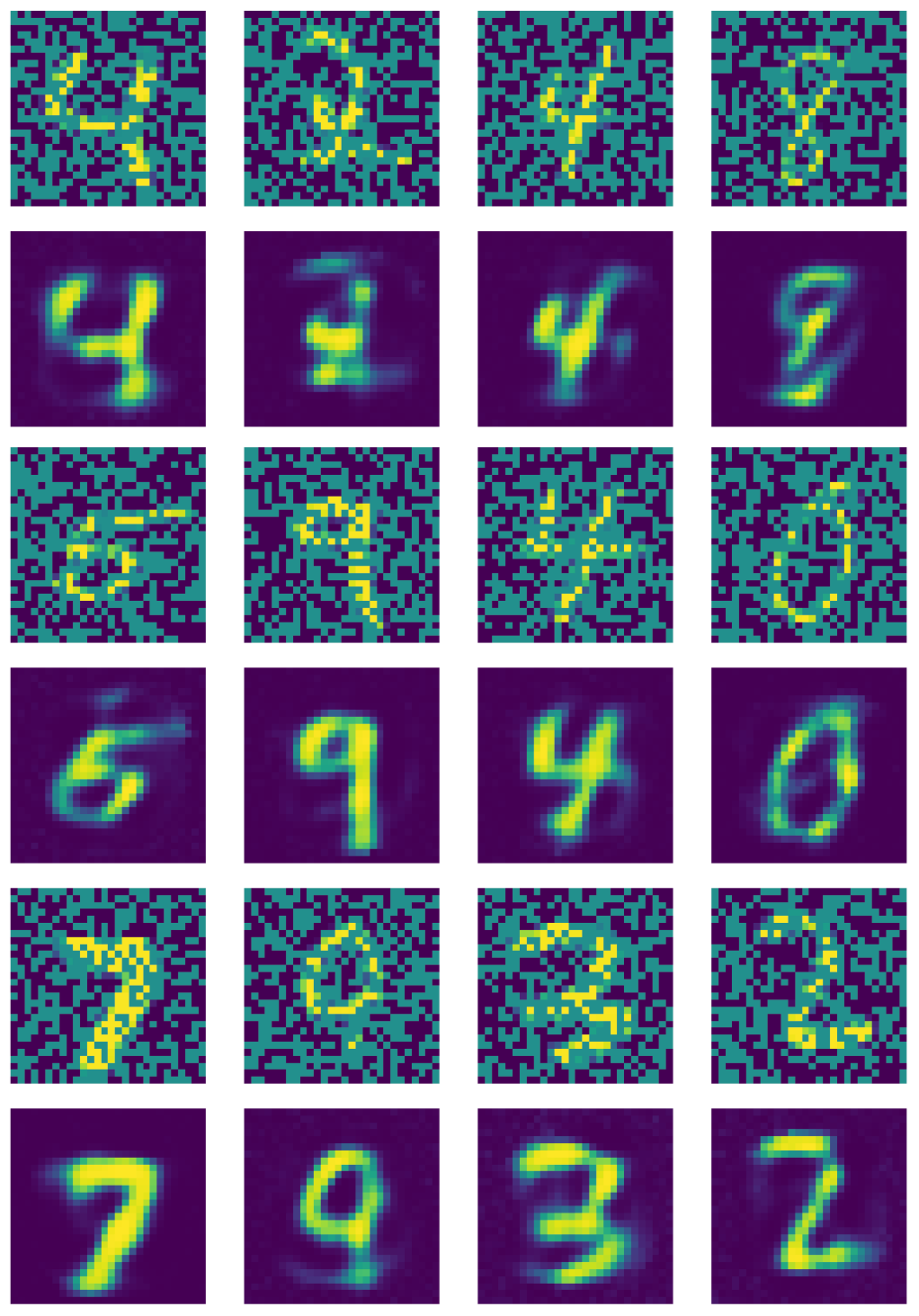
Fig. 21: Output of denoising autoencoder

Kernels comparison

It is important to note that in spite of the fact that the dimension of the input layer is $28 \times 28 = 784$, a hidden layer with a dimension of 500 is still an over-complete layer because of the number of black pixels in the image. Below are examples of kernels used in the trained under-complete standard autoencoder. Clearly, the pixels in the region where the number exists indicate the detection of some sort of pattern, while the pixels outside of this region are basically random. This indicates that the standard autoencoder does not care about the pixels outside of the region where the number is.

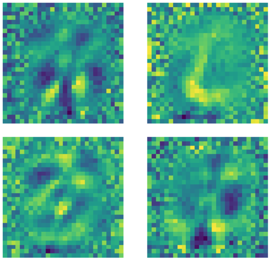
Figure 22: Standard AE kernels.

On the other hand, when the same data is fed to a denoising autoencoder where a dropout mask is applied to each image before fitting the model, something different happens. Every kernel that learns a pattern sets the pixels outside of the region where the number exists to some constant value. Because a dropout mask is applied to the images, the model now cares about the pixels outside of the number’s region.

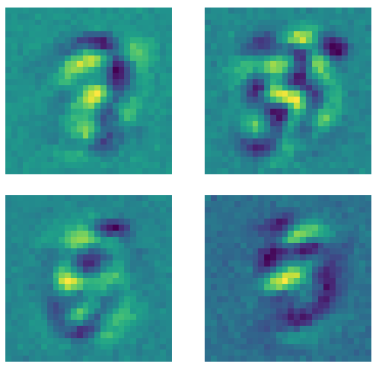
Figure 23: Denoising AE kernels.

Compared to the state of the art, our autoencoder actually does better!! You can see the results below.

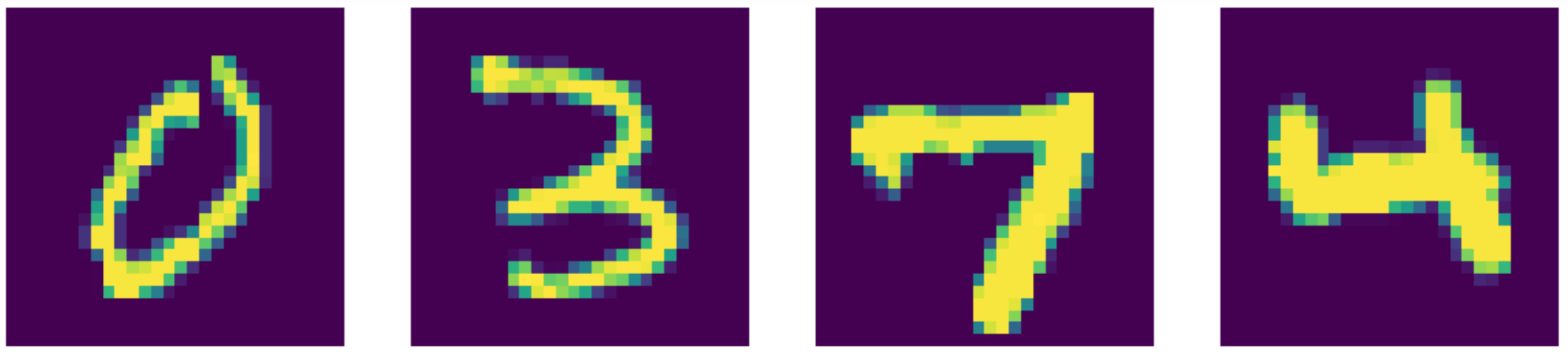
Figure 24: Input data (MNIST digits).

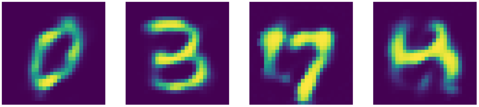
Figure 25: Denoising AE reconstructions.

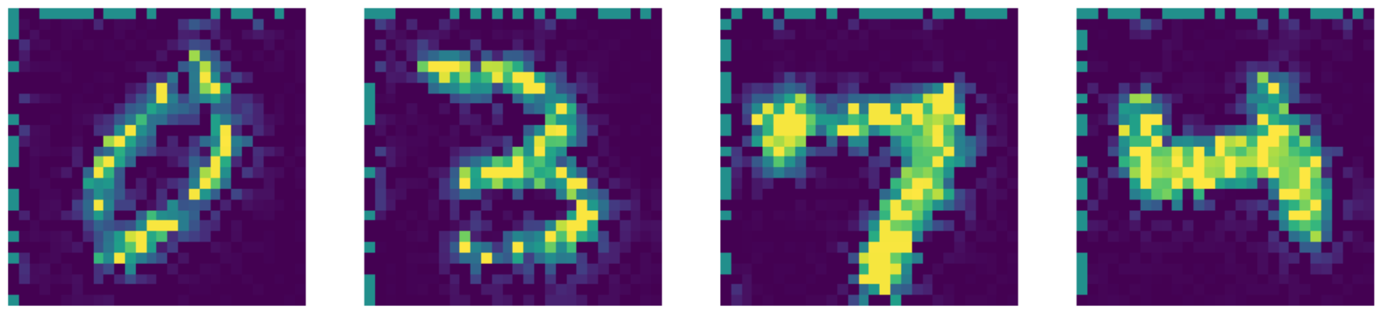
Figure 26: Telea inpainting output.

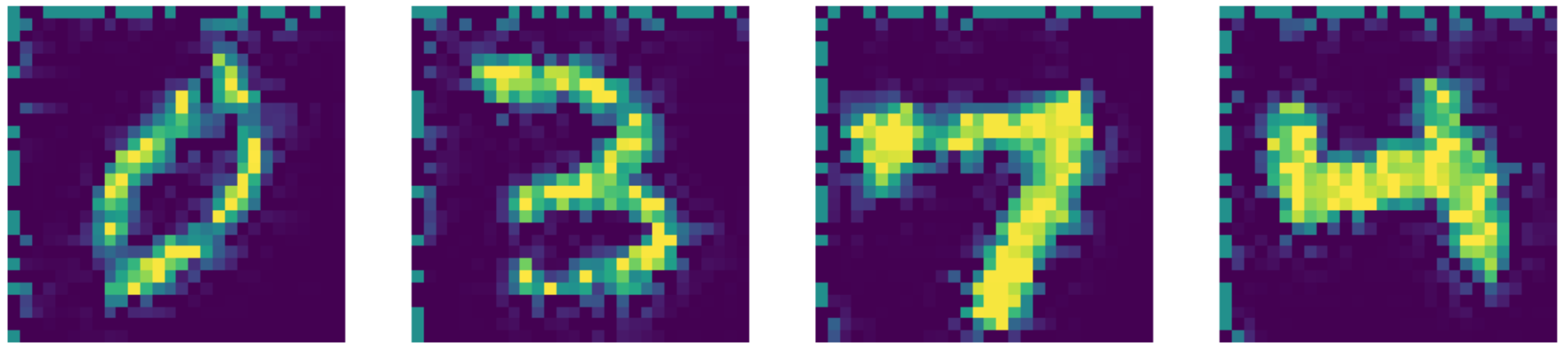
Figure 27: Navier-Stokes inpainting output.