Understanding convolutions and automatic differentiation engine

Understanding 1D convolution

In this part we will discuss convolution, since we would like to explore the sparsity, stationarity, compositionality of the data.

Instead of using the matrix $A$ discussed in the previous week, we will change the matrix width to the kernel size $k$. Therefore, each row of the matrix is a kernel. We can use the kernels by stacking and shifting (see Fig 1). Then we can have $m$ layers of height $n-k+1$.

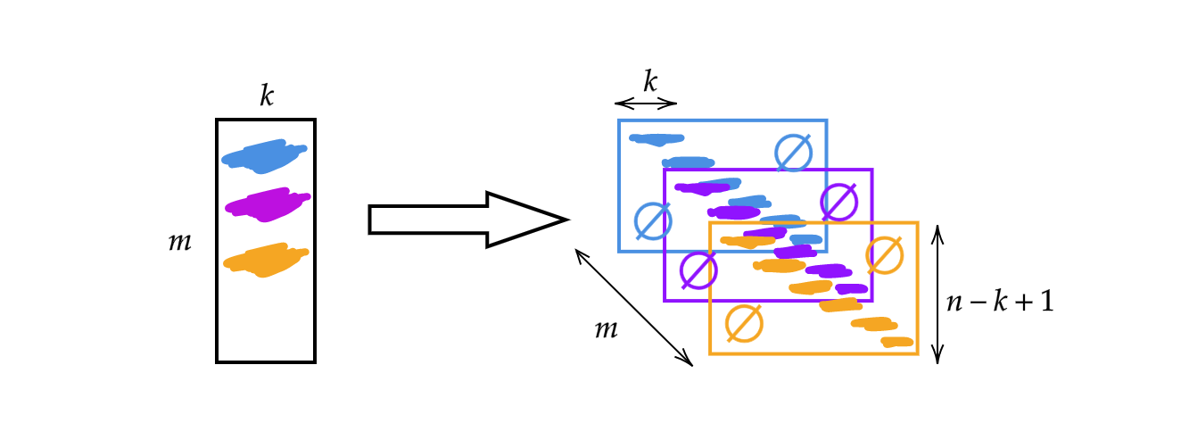
Fig 1: Illustration of 1D Convolution

The output is $m$ (thickness) vectors of size $n-k+1$.

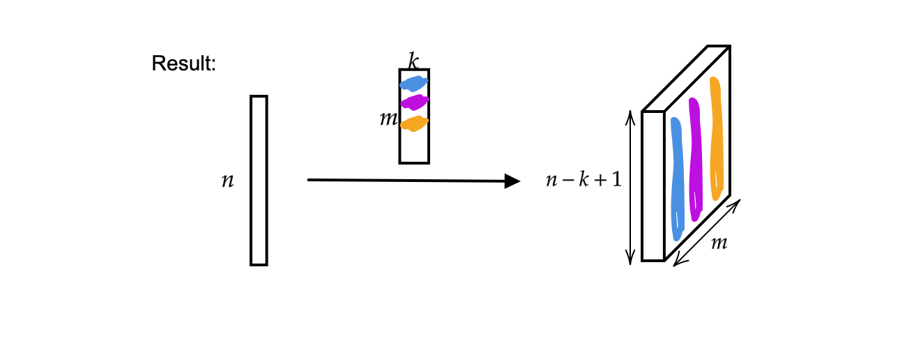
Fig 2: Result of 1D Convolution

Furthermore, a single input vector can viewed as a monophonic signal.

Fig 3: Monophonic Signal

Now, the input $x$ is a mapping

where $\Omega = \lbrace 1, 2, 3, \cdots \rbrace \subset \mathbb{N}^1$ (since this is $1$ dimensional signal / it has a $1$ dimensional domain) and in this case the channel number $c$ is $1$. When $c = 2$ this becomes a stereophonic signal.

For the 1D convolution, we can just compute the scalar product, kernel by kernel (see Fig 4).

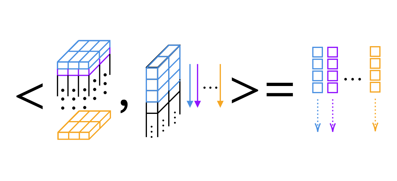
Fig 4: Layer-by-layer Scalar Product of 1D Convolution

Dimension of kernels and output width in PyTorch

Tips: We can use question mark in IPython to get access to the documents of functions. For example,

Init signature:
nn.Conv1d(
	in_channels,           # number of channels in the input image
	out_channels,          # number of channels produced by the convolution
	kernel_size,           # size of the convolving kernel
	stride=1,              # stride of the convolution
	padding=0,             # zero-padding added to both sides of the input
	dilation=1,            # spacing between kernel elements
	groups=1,              # nb of blocked connections from input to output
	bias=True,             # if `True`, adds a learnable bias to the output
	padding_mode='zeros',  # accepted values `zeros` and `circular`
)

1D convolution

We have $1$ dimensional convolution going from $2$ channels (stereophonic signal) to $16$ channels ($16$ kernels) with kernel size of $3$ and stride of $1$. We then have $16$ kernels with thickness $2$ and length $3$. Let’s assume that the input signal has a batch of size $1$ (one signal), $2$ channels and $64$ samples. The resulting output layer has $1$ signal, $16$ channels and the length of the signal is $62$ ($=64-3+1$). Also, if we output the bias size, we’ll find the bias size is $16$, since we have one bias per weight.

conv = nn.Conv1d(2, 16, 3)  # 2 channels (stereo signal), 16 kernels of size 3
conv.weight.size()          # output: torch.Size([16, 2, 3])
conv.bias.size()            # output: torch.Size([16])

x = torch.rand(1, 2, 64)    # batch of size 1, 2 channels, 64 samples
conv(x).size()              # output: torch.Size([1, 16, 62])

conv = nn.Conv1d(2, 16, 5)  # 2 channels, 16 kernels of size 5
conv(x).size()              # output: torch.Size([1, 16, 60])

2D convolution

We first define the input data as $1$ sample, $20$ channels (say, we’re using an hyperspectral image) with height $64$ and width $128$. The 2D convolution has $20$ channels from input and $16$ kernels with size of $3 \times 5$. After the convolution, the output data has $1$ sample, $16$ channels with height $62$ ($=64-3+1$) and width $124$ ($=128-5+1$).

x = torch.rand(1, 20, 64, 128)    # 1 sample, 20 channels, height 64, and width 128
conv = nn.Conv2d(20, 16, (3, 5))  # 20 channels, 16 kernels, kernel size is 3 x 5
conv.weight.size()                # output: torch.Size([16, 20, 3, 5])
conv(x).size()                    # output: torch.Size([1, 16, 62, 124])

If we want to achieve the same dimensionality, we can have paddings. Continuing the code above, we can add new parameters to the convolution function: stride=1 and padding=(1, 2), which means $1$ on $y$ direction ($1$ at the top and $1$ at the bottom) and $2$ on $x$ direction. Then the output signal is in the same size compared to the input signal. The number of dimensions that is required to store the collection of kernels when you perform 2D convolution is $4$.

# 20 channels, 16 kernels of size 3 x 5, stride is 1, padding of 1 and 2
conv = nn.Conv2d(20, 16, (3, 5), 1, (1, 2))
conv(x).size()  # output: torch.Size([1, 16, 64, 128])

How automatic gradient works?

In this section we’re going to ask torch to check all the computation over the tensors so that we can perform the computation of partial derivatives.

• Create a $2\times2$ tensor $\boldsymbol{x}$ with gradient-accumulation capabilities;
• Deduct $2$ from all elements of $\boldsymbol{x}$ and get $\boldsymbol{y}$; (If we print y.grad_fn, we will get <SubBackward0 object at 0x12904b290>, which means that y is generated by the module of subtraction $\boldsymbol{x}-2$. Also we can use y.grad_fn.next_functions[0][0].variable to derive the original tensor.)
• Do more operations: $\boldsymbol{z} = 3\boldsymbol{y}^2$;
• Calculate the mean of $\boldsymbol{z}$.

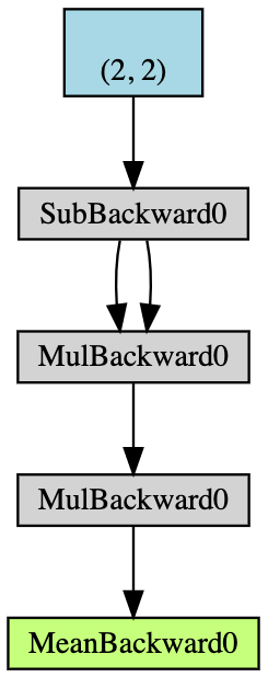
Fig 5: Flow Chart of the Auto-gradient Example

Back propagation is used for computing the gradients. In this example, the process of back propagation can be viewed as computing the gradient $\frac{d\boldsymbol{a}}{d\boldsymbol{x}}$. After computing $\frac{d\boldsymbol{a}}{d\boldsymbol{x}}$ by hand as a validation, we can find that the execution of a.backward() gives us the same value of x.grad as our computation.

Here is the process of computing back propagation by hand:

Whenever you use partial derivative in PyTorch, you get the same shape of the original data. But the correct Jacobian thing should be the transpose.

From basic to more crazy

Now we have a $1\times3$ vector $x$, assign $y$ to the double $x$ and keep doubling $y$ until its norm is smaller than $1000$. Due to the randomness we have for $x$, we cannot directly know the number of iterations when the procedure terminates.

x = torch.randn(3, requires_grad=True)

y = x * 2
i = 0
while y.data.norm() < 1000:
    y = y * 2
    i += 1

However, we can infer it easily by knowing the gradients we have.

gradients = torch.FloatTensor([0.1, 1.0, 0.0001])
y.backward(gradients)

print(x.grad)
tensor([1.0240e+02, 1.0240e+03, 1.0240e-01])
print(i)
9

As for the inference, we can use requires_grad=True to label that we want to track the gradient accumulation as shown below. If we omit requires_grad=True in either $x$ or $w$’s declaration and call backward() on $z$, there will be runtime error due to we do not have gradient accumulation on $x$ or $w$.

# Both x and w that allows gradient accumulation
x = torch.arange(1., n + 1, requires_grad=True)
w = torch.ones(n, requires_grad=True)
z = w @ x
z.backward()
print(x.grad, w.grad, sep='\n')

And, we can have with torch.no_grad() to omit the gradient accumulation.

x = torch.arange(1., n + 1)
w = torch.ones(n, requires_grad=True)

# All torch tensors will not have gradient accumulation
with torch.no_grad():
    z = w @ x

try:
    z.backward()  # PyTorch will throw an error here, since z has no grad accum.
except RuntimeError as e:
    print('RuntimeError!!! >:[')
    print(e)

More stuff – custom gradients

Also, instead of basic numerical operations, we can generate our own self-defined modules / functions, which can be plugged into the neural graph. The Jupyter Notebook can be found here.

To do so, we need to inherit torch.autograd.Function and override forward() and backward() functions. For example, if we want to training nets, we need to get the forward pass and know the partial derivatives of the input respect to the output, such that we can use this module in any kind of point in the code. Then, by using back-propagation (chain rule), we can plug the thing anywhere in the chain of operations, as long as we know the partial derivatives of the input respect to the output.

In this case, there are three examples of custom modules in the notebook, the add, split, and max modules. For example, the custom addition module:

# Custom addition module
class MyAdd(torch.autograd.Function):

    @staticmethod
    def forward(ctx, x1, x2):
        # ctx is a context where we can save
        # computations for backward.
        ctx.save_for_backward(x1, x2)
        return x1 + x2

    @staticmethod
    def backward(ctx, grad_output):
        x1, x2 = ctx.saved_tensors
        grad_x1 = grad_output * torch.ones_like(x1)
        grad_x2 = grad_output * torch.ones_like(x2)
        # need to return grads in order
        # of inputs to forward (excluding ctx)
        return grad_x1, grad_x2

If we have addition of two things and get an output, we need to overwrite the forward function like this. And when we go down to do back propagation, the gradients copied over both sides. So we overwrite the backward function by copying.

For split and max, see the code of how we overwrite forward and backward functions in the notebook. If we come from the same thing and Split, when go down doing gradients, we should add / sum them. For argmax, it selects the index of the highest thing, so the index of the highest should be $1$ while others being $0$. Remember, according to different custom modules, we need to overwrite its own forward pass and how they do gradients in backward function.