Optimisation Techniques II

Adaptive methods

SGD with momentum is currently the state of the art optimization method for a lot of ML problems. But there are other methods, generally called Adaptive Methods, innovated over the years that are particularly useful for poorly conditioned problems (if SGD does not work).

In the SGD formulation, every single weight in network is updated using an equation with the same learning rate (global $\gamma$). Here, for adaptive methods, we adapt a learning rate for each weight individually. For this purpose, the information we get from gradients for each weight is used.

Networks that are often used in practice have different structure in different parts of them. For instance, early parts of CNN may be very shallow convolution layers on large images and later in the network we might have convolutions of large number of channels on small images. Both of these operations are very different so a learning rate which works well for the beginning of the network may not work well for the latter sections of the network. This means adaptive learning rates by layer could be useful.

Weights in the latter part of the network (4096 in figure 1 below) directly dictate the output and have a very strong effect on it. Hence, we need smaller learning rates for those. In contrast, earlier weights will have smaller individual effects on the output, especially when initialized randomly.

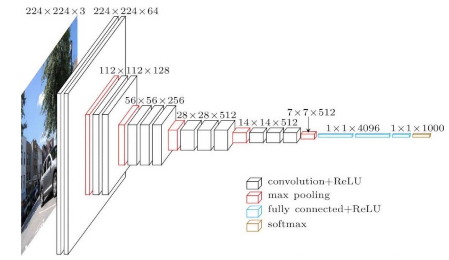
Figure 1: VGG16

RMSprop

The key idea of Root Mean Square Propagation is that the gradient is normalized by its root-mean-square.

In the equation below, squaring the gradient denotes that each element of the vector is squared individually.

where $\gamma$ is the global learning rate, $\epsilon$ is a value close to machine $\epsilon$ (on the order of $10^{-7}$ or $10^{-8}$) – in order to avoid division by zero errors, and $v_{t+1}$ is the 2nd moment estimate.

We update $v$ to estimate this noisy quantity via an exponential moving average (which is a standard way of maintaining an average of a quantity that may change over time). We need to put larger weights on the newer values as they provide more information. One way to do that is down-weight old values exponentially. The values in the $v$ calculation that are very old are down-weighted at each step by an $\alpha$ constant, which varies between 0 and 1. This dampens the old values until they are no longer an important part of the exponential moving average.

The original method keeps an exponential moving average of a non-central second moment, so we don’t subtract the mean here. The second moment is used to normalize the gradient element-wise, which means that every element of the gradient is divided by the square root of the second moment estimate. If the expected value of gradient is small, this process is similar to dividing the gradient by the standard deviation.

Using a small $\epsilon$ in the denominator doesn’t diverge because when $v$ is very small, the momentum is also very small.

ADAM

ADAM, or Adaptive Moment Estimation, which is RMSprop plus momentum, is a more commonly used method. The momentum update is converted to an exponential moving average and we don’t need to change the learning rate when we deal with $\beta$. Just as in RMSprop, we take an exponential moving average of the squared gradient here.

where $m_{t+1}$ is the momentum’s exponential moving average.

Bias correction that is used to keep the moving average unbiased during early iterations is not shown here.

Practical side

When training neural networks, SGD often goes in the wrong direction in the beginning of the training process, whereas RMSprop hones in on the right direction. However, RMSprop suffers from noise just as regular SGD, so it bounces around the optimum significantly once it’s close to a local minimizer. Just like when we add momentum to SGD, we get the same kind of improvement with ADAM. It is a good, not-noisy estimate of the solution, so ADAM is generally recommended over RMSprop.

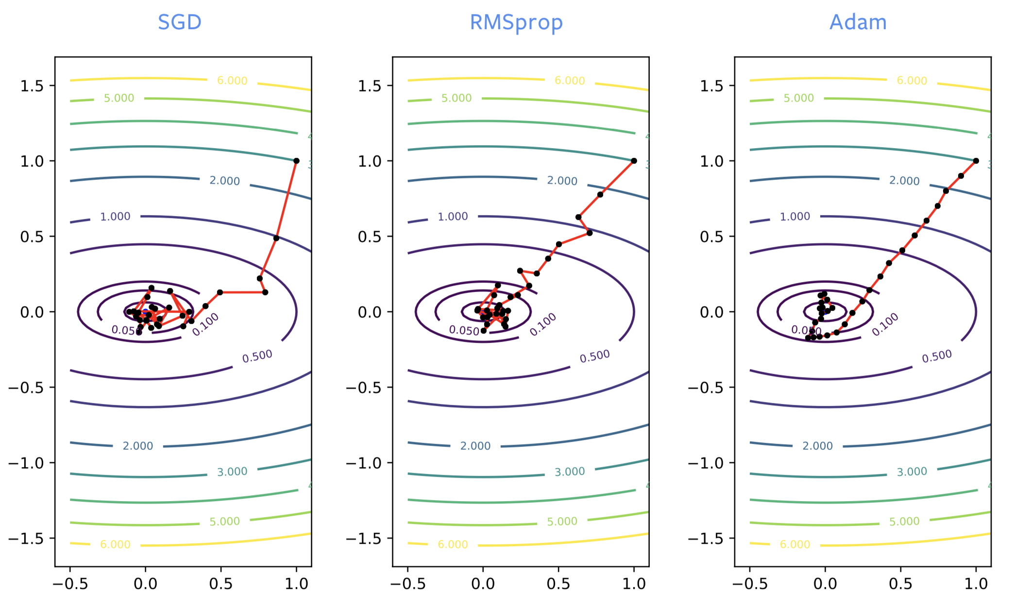
Figure 2: SGD *vs.* RMSprop *vs.* ADAM

ADAM is necessary for training some of the networks for using language models. For optimizing neural networks, SGD with momentum or ADAM is generally preferred. However, ADAM’s theory in papers is poorly understood and it also has several disadvantages:

• It can be shown on very simple test problems that the method does not converge.
• It is known to give generalization errors. If the neural network is trained to give zero loss on the data you trained it on, it will not give zero loss on other data points that it has never seen before. It is quite common, particularly on image problems, that we get worse generalization errors than when SGD is used. Factors could include that it finds the closest local minimum, or less noise in ADAM, or its structure, for instance.
• With ADAM we need to maintain 3 buffers, whereas SGD needs 2 buffers. This doesn’t really matter unless we train a model on the order of several gigabytes in size, in which case it might not fit in memory.
• 2 momentum parameters need to be tuned instead of 1.

Normalization layers

Rather than improving the optimization algorithms, normalization layers improve the network structure itself. They are additional layers in between existing layers. The goal is to improve the optimization and generalization performance.

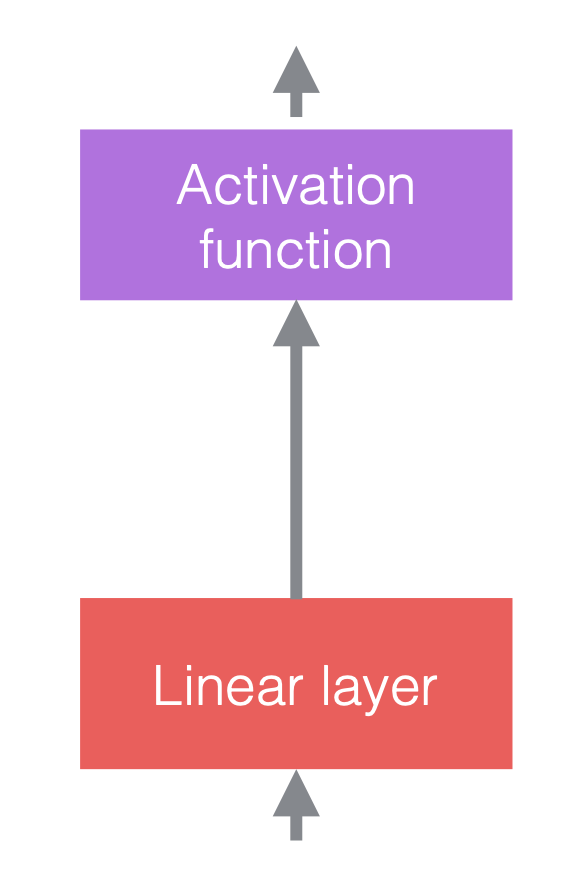
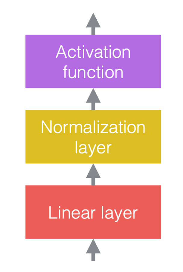
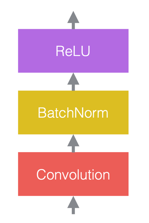
In neural networks, we typically alternate linear operations with non-linear operations. The non-linear operations are also known as activation functions, such as ReLU. We can place normalization layers before the linear layers, or after the activation functions. The most common practice is to put them between the linear layers and activation functions, as in the figure below.

(a) Before adding normalization	(b) After adding normalization	(c) An example in CNNs

In figure 3(c), the convolution is the linear layer, followed by batch normalization, followed by ReLU.

Note that the normalization layers affect the data that flows through, but they don’t change the power of the network in the sense that, with proper configuration of the weights, the unnormalized network can still give the same output as a normalized network.

Normalization operations

This is the generic notation for normalization:

where $x$ is the input vector, $y$ is the output vector, $\mu$ is the estimate of the mean of $x$, $\sigma$ is the estimate of the standard deviation (std) of $x$, $a$ is the learnable scaling factor, and $b$ is the learnable bias term.

Without the learnable parameters $a$ and $b$, the distribution of output vector $y$ will have fixed mean 0 and std 1. The scaling factor $a$ and bias term $b$ maintain the representation power of the network,i.e.the output values can still be over any particular range. Note that $a$ and $b$ do not reverse the normalization, because they are learnable parameters and are much more stable than $\mu$ and $\sigma$.

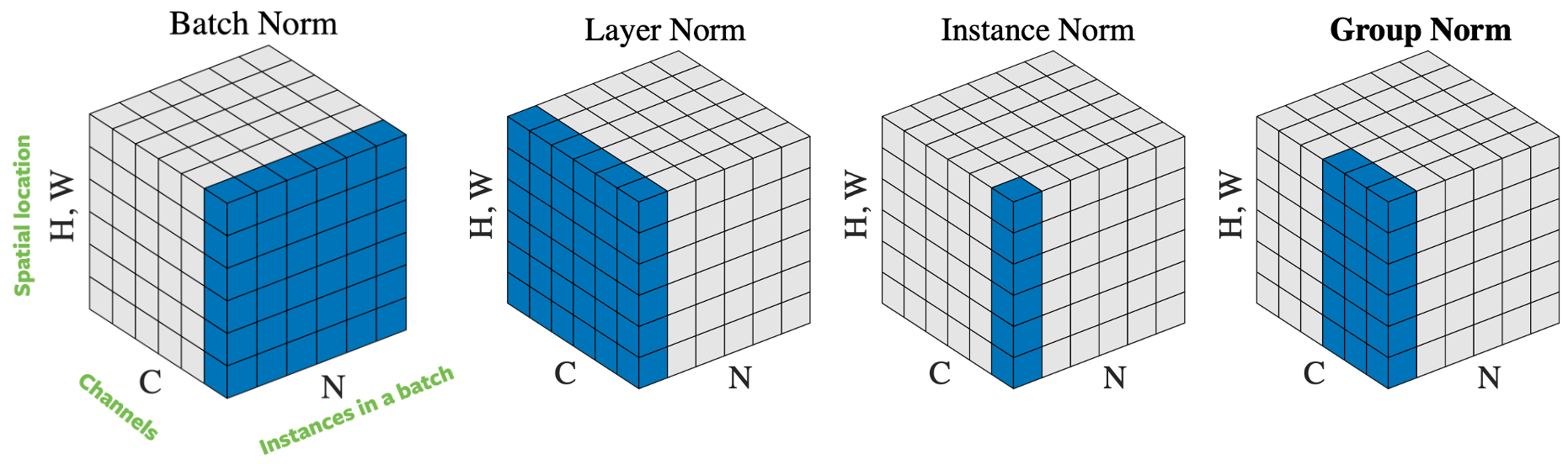
Figure 4: Normalization operations.

There are several ways to normalize the input vector, based on how to select samples for normalization. Figure 4 lists 4 different normalization approaches, for a mini-batch of $N$ images of height $H$ and width $W$, with $C$ channels:

• Batch norm: the normalization is applied only over one channel of the input. This is the first proposed and the most well-known approach. Please read How to Train Your ResNet 7: Batch Norm for more information.
• Layer norm: the normalization is applied within one image across all channels.
• Instance norm: the normalization is applied only over one image and one channel.
• Group norm: the normalization is applied over one image but across a number of channels. For example, channel 0 to 9 is a group, then channel 10 to 19 is another group, and so on. In practice, the group size is almost always 32. This is the approach recommended by Aaron Defazio, since it has good performance in practice and it does not conflict with SGD.

In practice, batch norm and group norm work well for computer vision problems, while layer norm and instance norm are heavily used for language problems.

Why does normalization help?

Although normalization works well in practice, the reasons behind its effectiveness are still disputed. Originally, normalization is proposed to reduce “internal covariate shift”, but some scholars proved it wrong in experiments. Nevertheless, normalization clearly has a combination of the following factors:

• Networks with normalization layers are easier to optimize, allowing for the use of larger learning rates. Normalization has an optimization effect that speeds up the training of neural networks.
• The mean/std estimates are noisy due to the randomness of the samples in batch. This extra “noise” results in better generalization in some cases. Normalization has a regularization effect.
• Normalization reduces sensitivity to weight initialization.

As a result, normalization lets you be more “careless” – you can combine almost any neural network building blocks together and have a good chance of training it without having to consider how poorly conditioned it might be.

Practical considerations

It’s important that back-propagation is done through the calculation of the mean and std, as well as the application of the normalization: the network training will diverge otherwise. The back-propagation calculation is fairly difficult and error-prone, but PyTorch is able to automatically calculate it for us, which is very helpful. Two normalization layer classes in PyTorch are listed below:

torch.nn.BatchNorm2d(num_features, ...)
torch.nn.GroupNorm(num_groups, num_channels, ...)

Batch norm was the first method developed and is the most widely known. However, Aaron Defazio recommends using group norm instead. It’s more stable, theoretically simpler, and usually works better. Group size 32 is a good default.

Note that for batch norm and instance norm, the mean/std used are fixed after training, rather than re-computed every time the network is evaluated, because multiple training samples are needed to perform normalization. This is not necessary for group norm and layer norm, since their normalization is over only one training sample.

The Death of Optimization

Sometimes we can barge into a field we know nothing about and improve how they are currently implementing things. One such example is the use of deep neural networks in the field of Magnetic Resonance Imaging (MRI) to accelerate MRI image reconstruction.

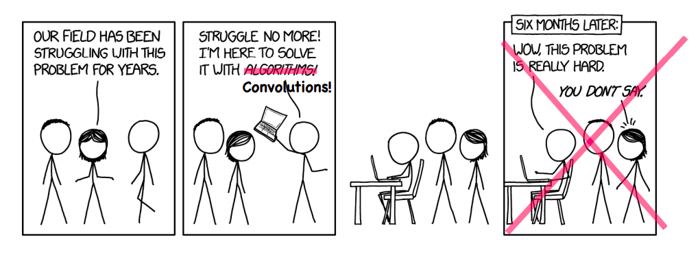
Figure 5: Sometimes it actually works!

MRI Reconstruction

In the traditional MRI reconstruction problem, raw data is taken from an MRI machine and an image is reconstructed from it using a simple pipeline/algorithm. MRI machines capture data in a 2-dimensional Fourier domain, one row or one column at a time (every few milliseconds). This raw input is composed of a frequency and a phase channel and the value represents the magnitude of a sine wave with that particular frequency and phase. Simply speaking, it can be thought of as a complex valued image, having a real and an imaginary channel. If we apply an inverse Fourier transform on this input, i.e add together all these sine waves weighted by their values, we can get the original anatomical image.

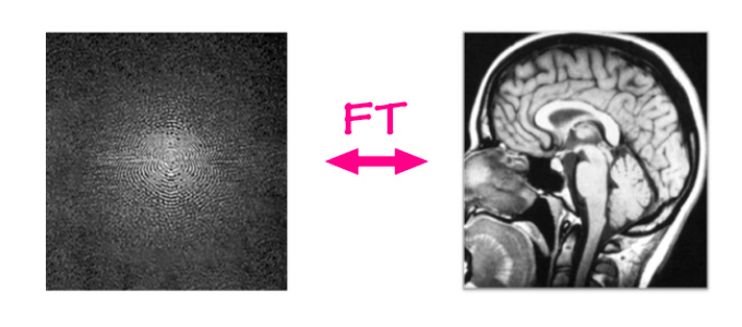
Fig. 6: MRI reconstruction

A linear mapping currently exists to go from the Fourier domain to the image domain and it’s very efficient, literally taking milliseconds, no matter how big the image is. But the question is, can we do it even faster?

Accelerated MRI

The new problem that needs to be solved is accelerated MRI, where by acceleration we mean making the MRI reconstruction process much faster. We want to run the machines quicker and still be able to produce identical quality images. One way we can do this and the most successful way so far has been to not capture all the columns from the MRI scan. We can skip some columns randomly, though it’s useful in practice to capture the middle columns, as they contain a lot of information across the image, but outside them we just capture randomly. The problem is that we can’t use our linear mapping anymore to reconstruct the image. The rightmost image in Figure 7 shows the output of a linear mapping applied to the subsampled Fourier space. It’s clear that this method doesn’t give us very useful outputs, and that there’s room to do something a little bit more intelligent.

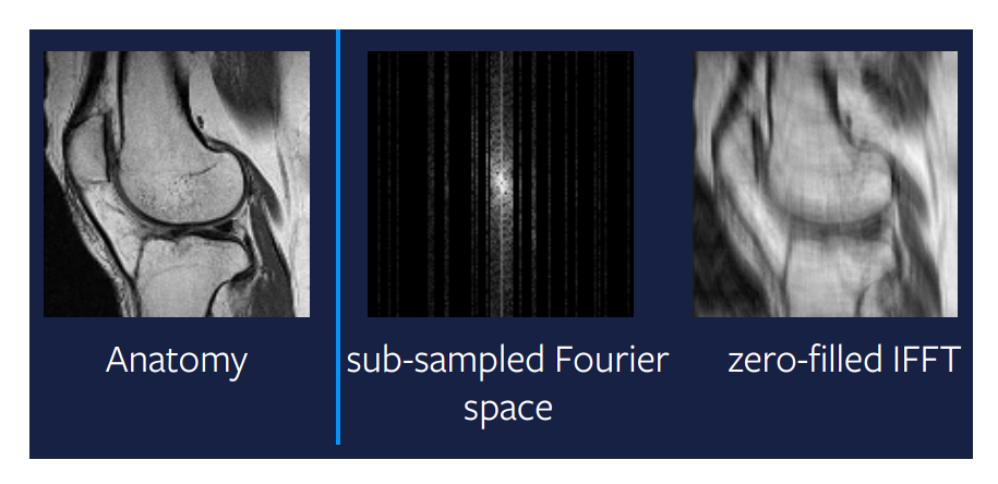
Fig.: Linear mapping on subsampled Fourier-space

Compressed sensing

One of the biggest breakthroughs in theoretical mathematics for a long time was compressed sensing. A paper by Candes et al. showed that theoretically, we can get a perfect reconstruction from the subsampled Fourier-domain image. In other words, when the signal we are trying to reconstruct is sparse or sparsely structured, then it is possible to perfectly reconstruct it from fewer measurements. But there are some practical requirements for this to work – we don’t need to sample randomly, rather we need to sample incoherently – though in practice, people just end up sampling randomly. Additionally, it takes the same time to sample a full column or half a column, so in practice we also sample entire columns.

Another condition is that we need to have sparsity in our image, where by sparsity we mean a lot of zeros or black pixels in the image. The raw input can be represented sparsely if we do a wavelength decomposition, but even this decomposition gives us an approximately sparse and not an exactly sparse image. So, this approach gives us a pretty good but not perfect reconstruction, as we can see in Figure 8. However, if the input were very sparse in the wavelength domain, then we would definitely get a perfect image.

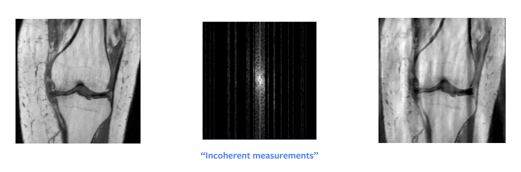
Figure 8: Compressed sensing

Compressed sensing is based on the theory of optimization. The way we can get this reconstruction is by solving a mini-optimization problem which has an additional regularization term:

where $M$ is the mask function that zeros out non-sampled entries, $\mathcal{F}$ is the Fourier transform, $y$ is the observed Fourier-domain data, $\lambda$ is the regularization penalty strength, and $V$ is the regularization function.

The optimization problem must be solved for each time step or each “slice” in an MRI scan, which often takes much longer than the scan itself. This gives us another reason to find something better.

Who needs optimization?

Instead of solving the little optimization problem at every time step, why not use a big neural network to produce the required solution directly? Our hope is that we can train a neural network with sufficient complexity that it essentially solves the optimization problem in one step and produces an output that is as good as the solution obtained from solving the optimization problem at each time step.

where $B$ is our deep learning model and $y$ is the observed Fourier-domain data.

15 years ago, this approach was difficult – but nowadays this is a lot easier to implement. Figure 9 shows the result of a deep learning approach to this problem and we can see that the output is much better than the compressed sensing approach and looks very similar to the actual scan.

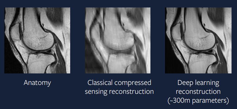
Figure 9: Deep Learning approach

The model used to generate this reconstruction uses an ADAM optimizer, group-norm normalization layers, and a U-Net based convolutional neural network. Such an approach is very close to practical applications and we will hopefully be seeing these accelerated MRI scans happening in clinical practice in a few years’ time. –>