Transformer Encoder-predictor-decoder architecture

The Transformer

Before elaborating the encoder-predictor-decoder architecture, we are going to review two models we’ve seen before.

Conditional EBM latent variable architecture

We should be familiar with the terminology of these modules from the previous lectures. In the conditional EBM latent variable architecture, we have $x$ the conditional variable which goes into a predictor. We have $\vy$ which is the target value. The decoder modules will produce $\vytilde$ when fed with a latent variable $z$ and the output of the predictor. $\red{E}$ is the energy function which minimizes the energy between $\vytilde$ and $\vy$.

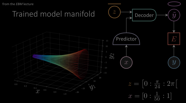
Figure 1: (From the EBM lecture) Diagram above depicting the architecture of a conditional EBM latent variable model.

Autoencoder architecture

In Autoencoder architecture , we observed there is no conditional input but only a target variable. The entire architecture is trying to learn the structure in these target variables. The target value $\vy$ is fed through an encoder module which transforms into a hidden representation space, forcing only the most important information through. And the decoder will make these variables come back to the original target space with a $\vytilde$. And the cost function will try to minimize the distance between $\vytilde$ and $\vy$.

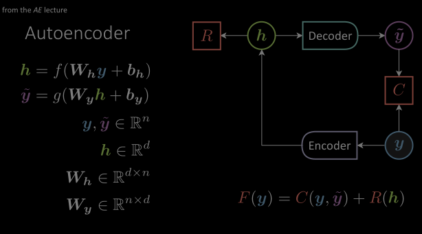
Figure 2: (From the autoencoder lecture) Architecture of a basic Autoencoder consisting of encoder and decoder modules.

Encoder-predictor-decoder architecture

Figure 3: The transformer architecture with a unit delay module.

In a transformer, $\vy$ (target sentence) is a discrete time signal. It has discrete representation in a time index. The $\vy$ is fed into a unit delay module succeeded by an encoder. The unit delay here transforms $\vy[j] \mapsto \vy[j-1]$. The only difference with the autoencoder here is this delayed variable. So we can use this structure in the language model to produce the future when given the past.

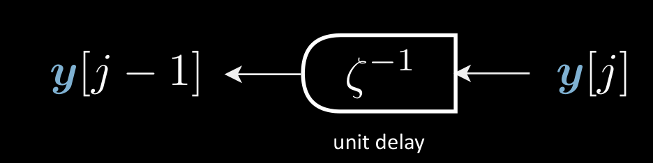
Figure 4: A unit delay module transforms $\vy[j] \mapsto \vy[j-1]$

The observed signal, $\vx$ (source sentence) , is also fed through an encoder. The output of both encoder and delayed encoder are fed into the predictor, which gives a hidden representation $\vh$. This is very similar to denoising autoencoder as the delay module acts as noise in this case. And $\vx$ here makes this entire architecture a conditional delayed denoising autoencoder.

Encoder module

You can see the detailed explanation of these modules from last year’s slides here.

Predictor Module

The transformer predictor module follows a similar procedure as the encoder. However, there is one additional sub-block (i.e. cross-attention) to take into account. Additionally, the output of the encoder modules acts as the inputs to this module.

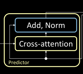
Figure 5: The predictor module consisting of a cross attention block

Cross attention

You can see the detailed explanation of cross attention from last year’s slides cross-attention.

Decoder module

Contrary to what authors of the Transformer paper define, the decoder module consists of 1D-convolution and Add, Norm blocks. The output of the predictor module is fed to the decoder module and the output of the decoder module is the predicted sentence. We can train this by providing the delayed target sequence.

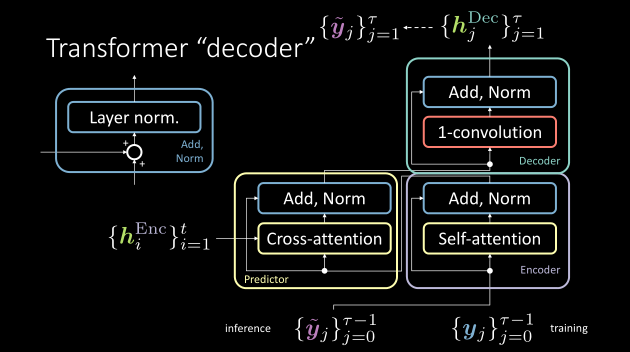
Figure 6: The correct notation of the encoder,predictor and decoder modules in a transformer