Introduction to Autoencoders

Applications of Autoencoder

DALL-E: Creating Images from Text

DALL-E (released by OpenAI) is a neural network based on the Transformers architecture, that creates images from text captions. It is a 12-billion parameter version of GPT-3, trained on a dataset of text-image pairs.

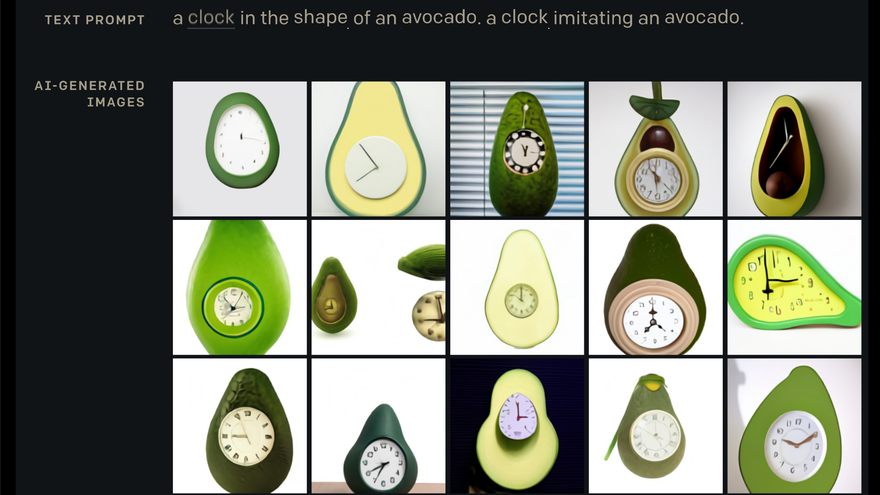
Figure 1: DALL-E: Input-Output

Go to the website and play with the captions!

Autoencoder

Let’s start with some definitions:

Definitions

Input

$\vx$: is observed during both training and testing

$\vy$: is observed during training but not testing

$\vz$: is not observed (neither during training nor during testing).

Output

$\vh$: is computed from the input (hidden/internal)

$\vytilde$: is computed from the hidden (predicted $\vy$, ~ means circa)

Confused? Refer to the below figure to understand the use of different variables in different machine learning techniques.

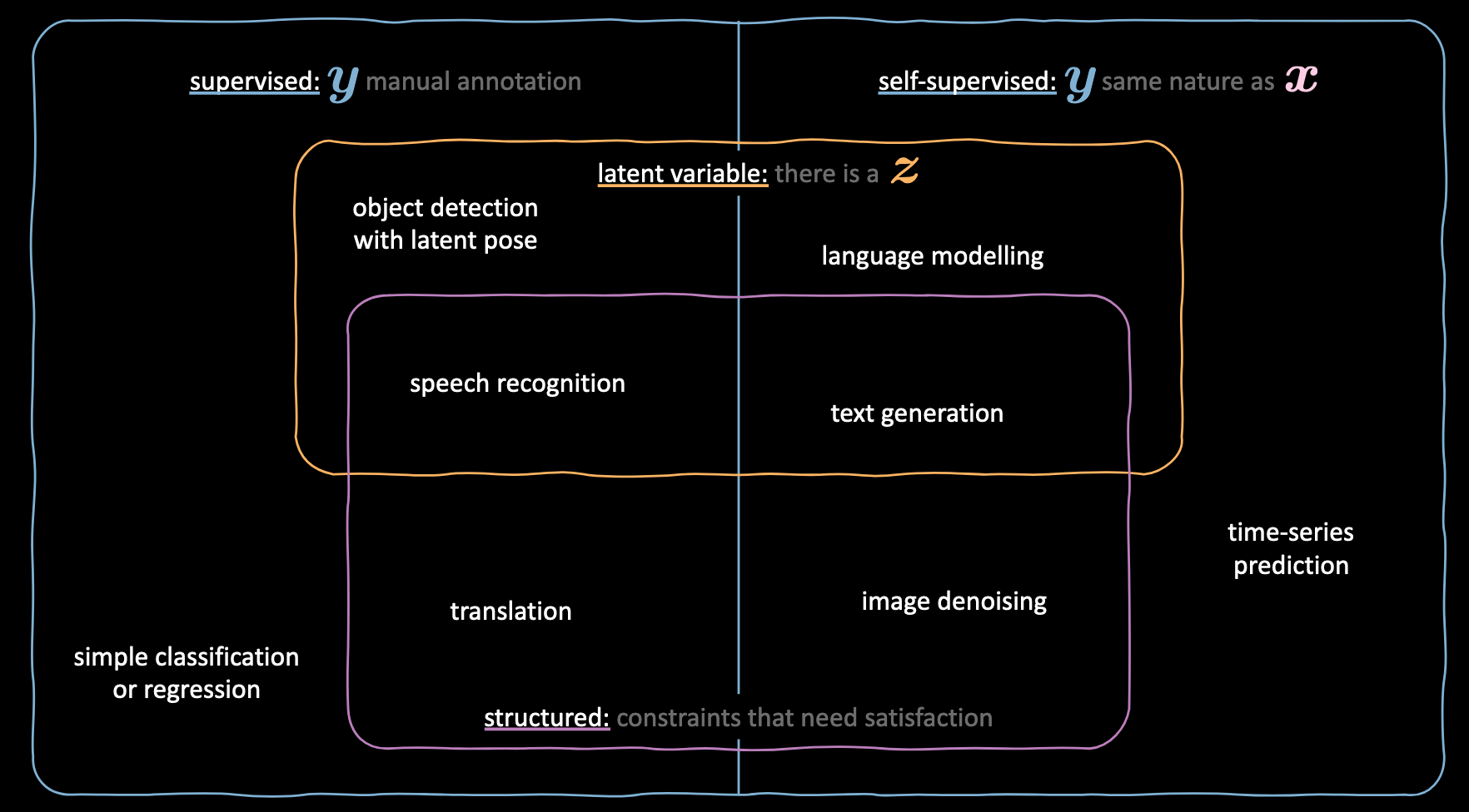
Figure 2: Variable definitions in different machine learning techniques

Introduction

These kinds of networks are used to learn the internal structure of some input and encode it in a hidden internal representation $\vh$, which expresses the input.

We already learned how to train energy-based models, let’s look at the below network:

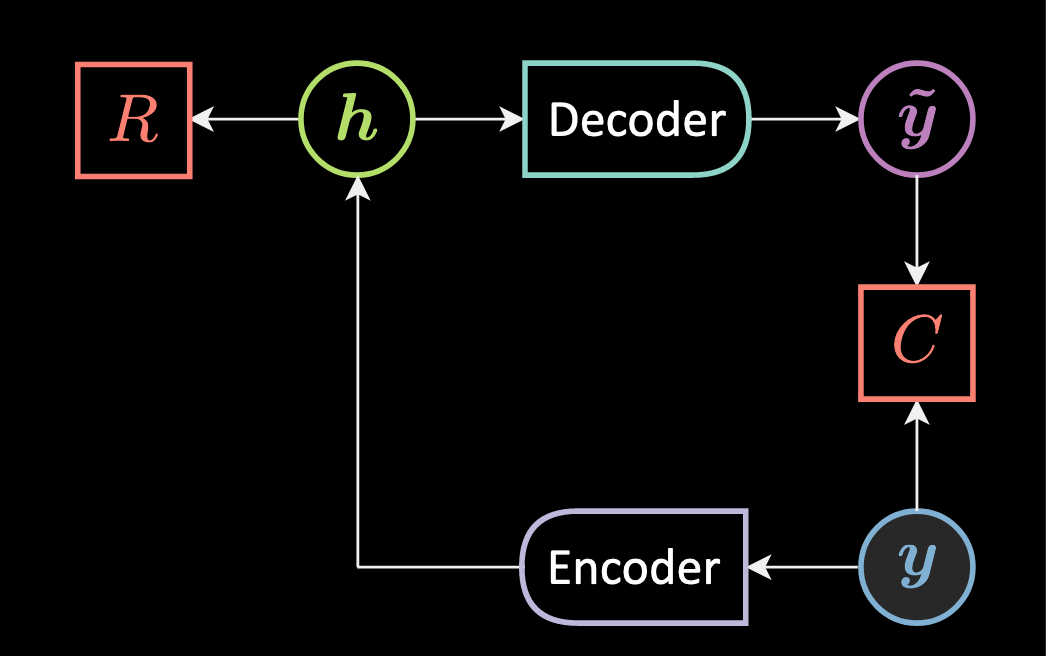
Figure 3: Autoencoder Architecture

Here instead of computing the minimization of the energy $\red{E}$ for $\vz$, we use an encoder that approximates the minimization and provides a hidden representation $\vh$ for a given $\vy$.

Then the hidden representation is convected into $\vytilde$ (Here we don’t have a predictor, we have an encoder).

Basically, $\vh$ is the output of a squashing function $f$ of the rotation of our input/observation $\vy$. $\vytilde$ is the output of squashing function $g$ of the rotation of our hidden representation $\vh$.

Note that, here $\vy$ and $\vytilde$ both belong to the same input space, and $\vh$ belong to $\mathbb{R}^d$ which is the internal representation. $\mW_h$ and $\mW_y$ are matrices for rotation.

This is called Autoencoder. The encoder is performing amortizing and we don’t have to minimize the energy $\red{E}$ but $\red{F}$:

Reconstruction Costs

Below are the two examples of reconstruction energies:

Real-Valued Input:

This is the square euclidean distance between $\vy$ and $\vytilde$.

Binary input

In the case of binary input, we can simply use binary cross-entropy

Loss Functionals

Average across all training samples of per sample loss function

We take the energy loss and try to push the energy down on $\vytilde$

Use-cases

The size of the hidden representation $\vh$ obtained using these networks can be both smaller and larger than the input size.

If we choose a smaller $\vh$, the network can be used for non-linear dimensionality reduction.

In some situations it can be useful to have a larger than input $\vh$, however, in this scenario, a plain autoencoder would collapse. In other words, since we are trying to reconstruct the input, the model is prone to copying all the input features into the hidden layer and passing it as the output thus essentially behaving as an identity function. This needs to be avoided as this would imply that our model fails to learn anything.

To prevent the model from collapsing, we have to employ techniques that constrain the amount of region which can take zero or low energy values. These techniques can be some sort of regularization such as sparsity constraints, adding additional noise, or sampling.

Denoising autoencoder

We add some augmentation/corruption like Gaussian noise to an input sampled from the training manifold $\vyhat$ before feeding it into the model and expect the reconstructed input $\vytilde$ to be similar to the original input $\vy$.

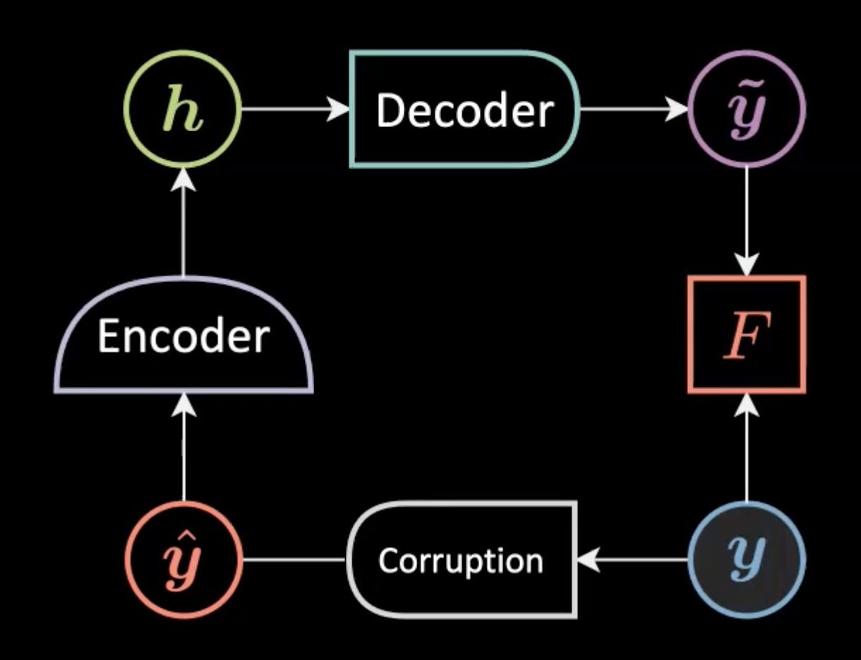
Figure 4: Denoising Autoencoder Network architecture.

An important note: The noise added to the original input should be similar to what we expect in reality, so the model can easily recover from it.

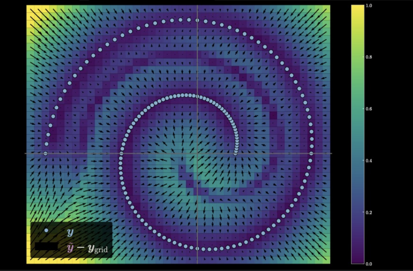
Figure 5: Measuring the traveling distance of the input data

In the image above, the light colour points on the spiral represent the original data manifold. As we add noise, we go farther from the original points. These noise-added points are fed into the auto-encoder to generate this graph. The direction of each arrow points to the original datapoint the model pushes the noise-added point towards; whereas the size of the arrow shows by how much. We also see a dark purple spiral region which exists because the points in this region are equidistant from two points on the data manifold.