Low Resource Machine Translation II

We start with standard machine learning algorithms can be applied in the realm of machine translation translation. Then, we take a deeper look into understanding different perspectives on this application. Our setting consists of multiple languages and multiple domains, but eventually we want to maximize translation accuracy of a certain domain in a language class.

NLP/MT Data

• Parallel dataset
• monolingual Data
• Multiple language pairs
• Multiple Domains

ML Techniques

• Supervised learning
• Semi-supervised Learning
• Multi-task/multi-modal learning
• Domain adaptation

Taking a deeper look at the type of data we are presented with in machine translation, we can better understand how these applications can be mapped to machine learning techniques. For example, if we have a parallel dataset in the space of machine translation, then we have its equivalent in supervised learning. Second, we could have monolingual data in machine translation–this translates to semi-supervised learning within the machine learning framework. Third, if we have multiple language paris in machine translation, we can closely compare this to multi-task learning within the ML space. And lastly, if we have multiple domains in machine translation, we can compare this to domain adaptation in machine learning. When you have many domains, you naturally also want to use different domain adaptation techniques

Case Studies

Translating from English to Nepali: Let’s start with a simple case study within the realm of supervised learning. For example, let’s say that we have a sentence in English and we want to translate it to Nepali. This is similar to multitask learning in the sense that you have one task, and then you add another task you’re interested in. Since we have multiple domains we can start thinking about domain adaptation techniques and analyzing which domain adaptation techniques are applicable to machine translation.

We can define our supervised learning method as the following when translating from English to Nepali:

Our per-sample loss using the usual attention-based transformer is defined as the following:

We can regularize the model using:

• Dropout
• Label Smoothing

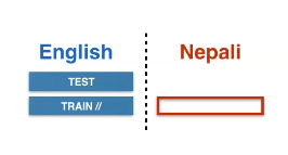
Figure 1: Supervised Learning from English to Nepali

Beginning with a supervised learning setting, we can use the aforementioned example of translation. Our dataset is

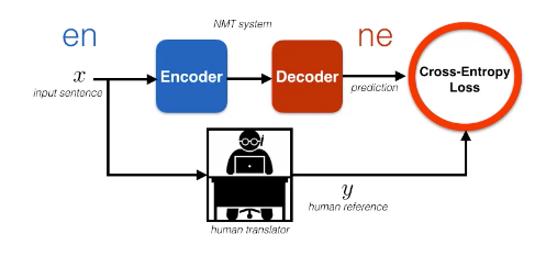
Figure 2: Supervised Learning Visualization

We can train this model using maximum likelihood, where we want to maximize ${ \vy\vert \vx } $.

One way to represent this methodology is by the diagram, where you have a blue encoder that processes English sentences, and a red decoder that processes Nepali. From here, we want to compute our cross-entropy loss and update our model parameters. We may also want to regularize the model using either dropout or label smoothing. Additionally, we may need to regularize using the log loss

Note: Transliteration is not word per word translation. It means that you’re using the characters from one language to make a logical translation of the word in a different language.

How can we improve generalization?

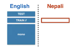
Figure 3: Semi-Supervised Learning (DAE) from English to Nepali

We can get additional source side monolingual data with this approach as well.

When using the DAE learning framework, we an either pre-train or add a DAE loss to the supervised cross entropy term:

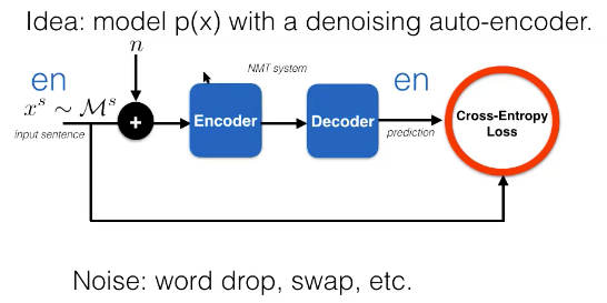
Figure 4: Semi-Supervised Learning (DAE) Diagram

One way to leverage an additional dataset is by trying to model $p(\vx)$ with a semi-supervised approach. One way to model \(p(\vx)\) is via the denoising of an auto-encoder. This is particularly useful because the encoder and decoder share a similar machine translation methodology. In the semi-supervised learning approach, going from English to Nepali, we have:

And when we want to predict missing labels using decoding and training noise, we can use cross-entropy loss as such:

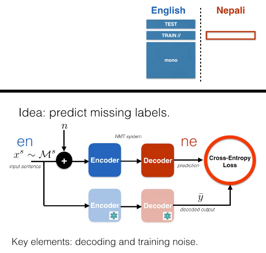
Figure 5: Semi-Supervised Learning (ST)

Another approach would be via self-training or pseudolearning. This is an algorithm from the 90s and the idea is that you take your sentence from the monolingual dataset and then you inject noise to it, you encode the poor translation you made and then make a prediction to produce the desired outcome. You can tune the parameters by minimizing the standard cross entropy loss on the labeled data. In other words, we are minimizing $L^{\sup} (\vtheta) + \lambda L^\text{ST} \vtheta$. We are basically using a stale version of our model to produce the desired output $\vy$.

ALGORITHM

• train model $p(\vy \mid \vx)$ on $\red{D}$
• repeat
  • decode $\vx^s \sim \mathcal{M}^s$ to $\bar{\vy}$ and create additional dataset \(\mathcal{A}^s = \{(\vx^s_j,\vy_j\}_{j=1,\vect{...},M_s})\)
  • retrain model on: $\mathcal{D} \cup \mathcal{A}^s$

This method works because: (1) when we produce $\vy$, we typically trying to learn the search procedure (2) we insert noise which creates smoothing for the output space

Working with monolingual data: If we are working on the other hand with monolingual data, first we would need to train a reverse machine learning translation system of backward machines.

Two benefits from adding target-side monolingual data

• Decoder learns a good language model
• Better generalization via data augmentation

The algorithm would stay the same as above, where we have smaller systems of encoders and decoders.

ALGORITHM

• train model $p(\vx\mid \vy)$ on $\mathcal{D}$
• decode $\vy^t \sim \mathcal{M}^t$ to $\vx$ with $p(\vx\mid \vy)$, and create additional dataset $\mathcal{A}^t = \lbrace ( \bar {\vx}_k,\vy^t_k \rbrace _{k=1,\vect{…},M_t})$
• retrain model $p(\vy\mid \vx)$ on: $\mathcal{D} \cup \mathcal{A}^t$

Finally, we can put these two algorithms together in an iterative process.

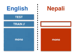
Figure 6: Semi-Supervised Learning Case Scenario

We can get additional source and target side monolingual data.

The process we can follow is via this algorithm:

• train model $p(\vx \mid \vy)$ and $p(\vy \mid \vx)$ on $\mathcal{D}$
• repeat
  • Phase 1
  • decode $\vy^{t} \sim \mathcal{M}^{t}$ to $\bar{\vx}$ with $p(\vx \mid \vy)$, create additional dataset
  \[\mathcal{A}^{t}=\left\{\left(\bar{\vx}_{k}, \vy_{k}^{t}\right)\right\}_{k=1, \ldots, M_{t}}\]
  • decode $\vx^{s} \sim \mathcal{M}^{s}$ to $\bar{\vy}$ with $p(\vy \mid \vx)$, create additional dataset
  \[\mathcal{A}^{s}=\left\{\left(\vx_{j}^{s}, \bar{\vy}_{j}\right)\right\}_{j=1, \ldots, M}\]
  • Phase 2
  • retrain both $p(\vy \mid \vx)$ and $p(\vx \mid \vy)$ on: \(\mathcal{D} \cup \mathcal{A}^{t} \cup \mathcal{A}^{s}\)
  \[\mathcal{L}^{\text {total }}(\vtheta)=-\log p(\vy \mid \vx)-\lambda_{1} \log p\left(\vy^{t} \mid \bar{\vx}^{t}\right)-\lambda_{2} \log p\left(\bar{\vy}^{s} \mid \vx^{s}\right)\]

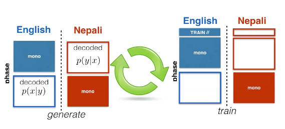
Figure 7: Semi-Supervised Learning Diagram (ST+BT)

Next question is how to deal with multiple languages

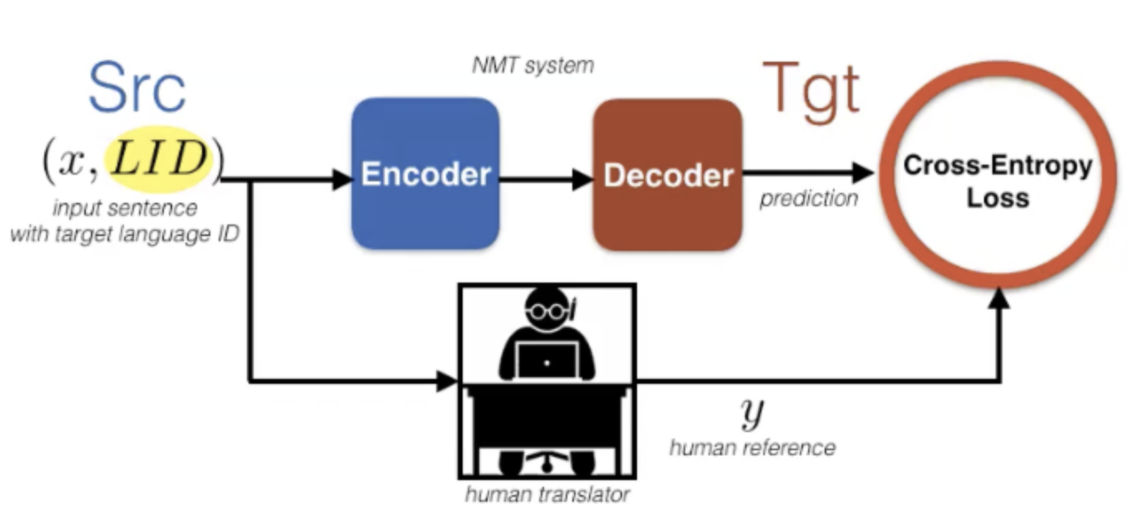
Figure 8: Semi-Supervised Learning Case Scenario on Multiple Languages

This is the learning framework for multilingual training, which shares encoder and decoder across all the language pairs, prepends a target language identifier to the source sentence to inform decoder of desired language and concatenates all the datasets together.

Mathematically, the train uses standard cross-entropy loss:

How do we deal with domain adaptation?

If you have small data in domain validation, what you can do is fine-tuning, which is super effective. Basically train on domain A and finetune on domain B by continuing training for a little bit on the validation set.

Unsupervised MT

Let’s consider English and French.

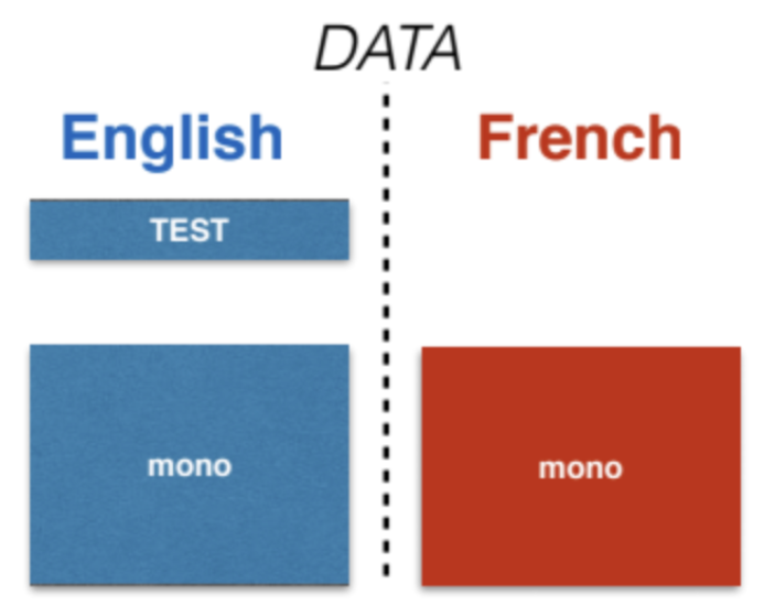
Figure 9: Unsupervised Machine Translation on English and French

Iterative BT

The following architecture first translate French to some random unknown English words. Since there is no ground truth reference, what could do is feeding this translation to another machine translation system goes from English to French. The problem here is lack of constrains on $\bar{\vx}$

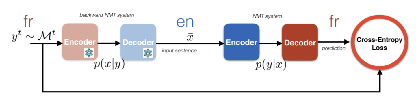
Figure 10: Iterative BT for English and French

DAE

DAE adds a constraint on the $\bar{\vect{x}}$ to make sure that decoder outputs fluently in the desired language. One way is adding denoising of the encoding turn to the loss function. This may not work since decoder may behave differently when fed with representations from French encoder vs English encoder (lack of modularity)

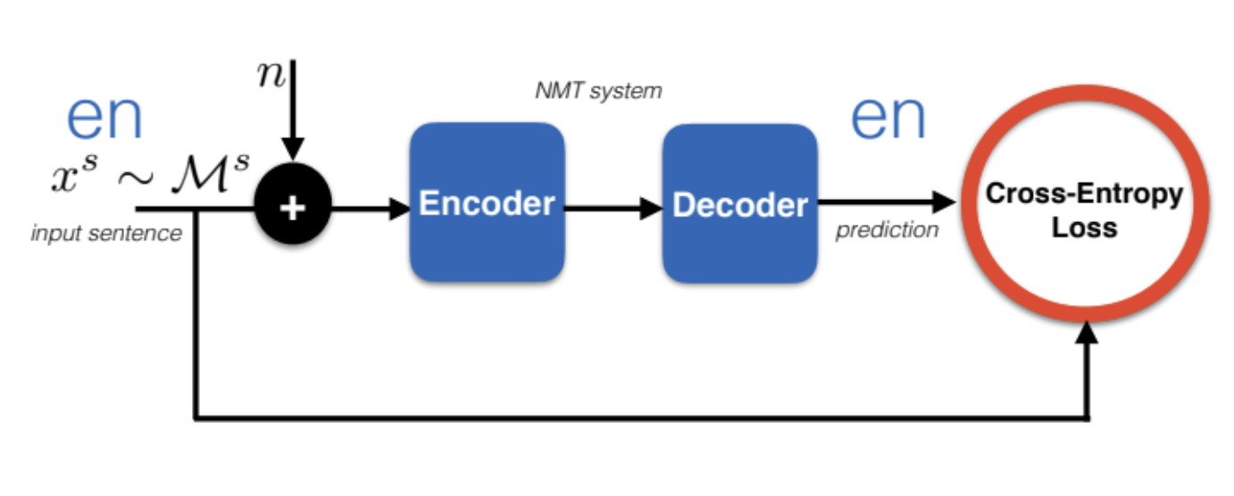
Figure 11: DAE

Multi-Lingual

One way to fix is by sharing all parameters of encoder and decoder so that the feature space share no matter whether you feed the French or English sentence (only one encoder and decoder now)

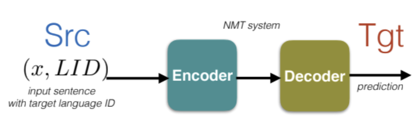
Figure 12: Multi-Lingual

BLEU score

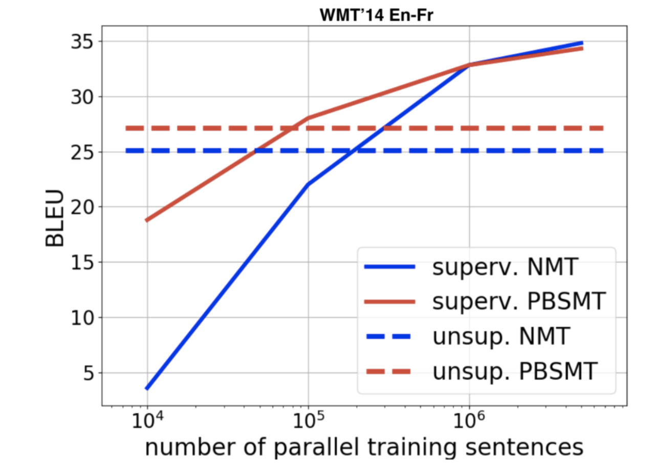
Figure 13: BLEU Score

This graph tells why machine translation is very large scale learning, because you need to compensate for the lack of direct supervision by adding more and more data.

FLoRes Ne-En

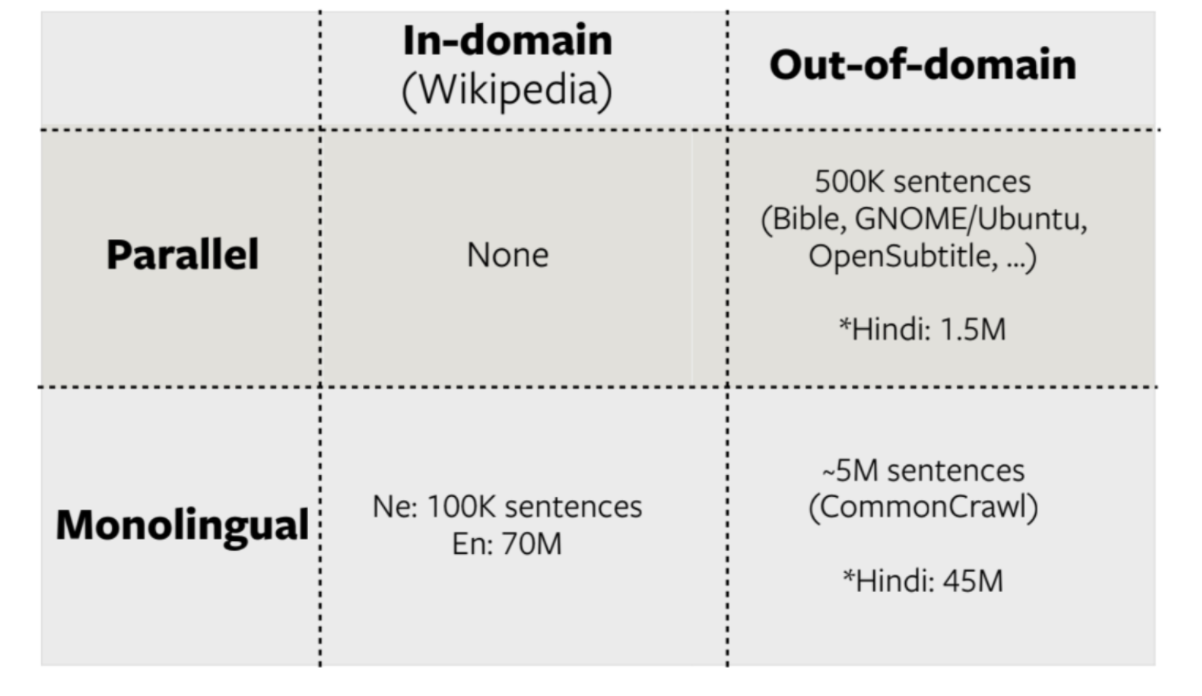
Figure 14: FLoRes Ne-En

Results on FLoRes: Ne-En

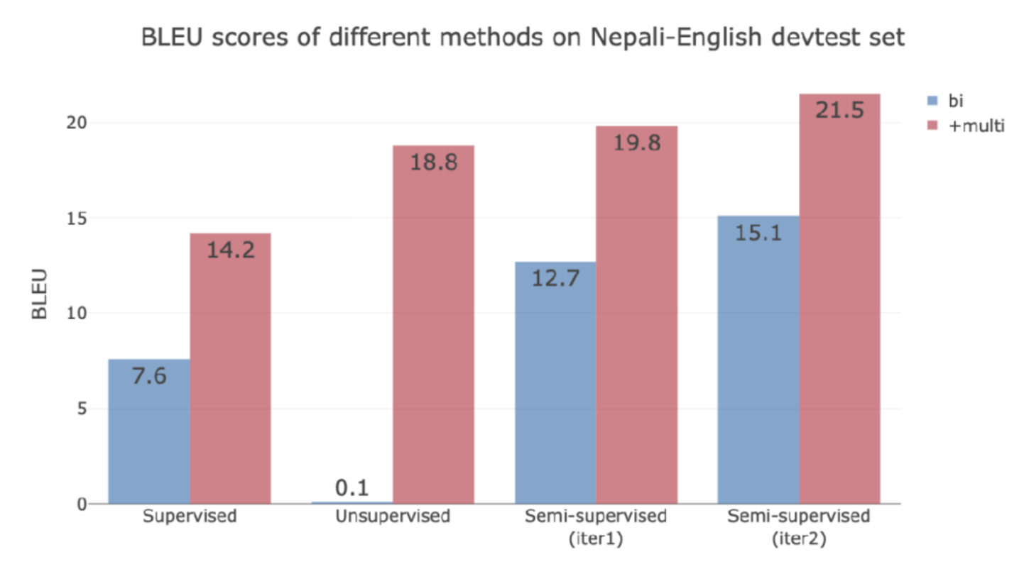
Figure 15: FLoRes Ne-En Results

The unsupervised learning doesn’t work at all in this case because two monolingual for the stats are from different domains and there is no way to find correspondences.

If adding English-Hindi data since Hindi and Nepali are similar, all four models dramatically improve (Red).

If you want to add language that is less related, you need to add so much. Since low-resource MT requires big data and big compute!

In conclusion, the less labeled data you have, the more data you need to use:

Supervised Learning

• Each datum yields X bits of information useful to solve the task
• Need N samples
• Need model of size YB.

Unsupervised Learning

• Each datum yields X/1000 bits
• Need N*1000 samples
• Need model of size Y*f(1000) MB.

Perspectives

Typically, in machine learning and machine translation, we always consider a domain mismatch between the training and the test distribution. When we have a slightly different domain, we need to do domain adaptation (e.g. domain tagging and finetuning). Here we will talk about a different domain mismatch which is:

Source-Target Domain Mismatch

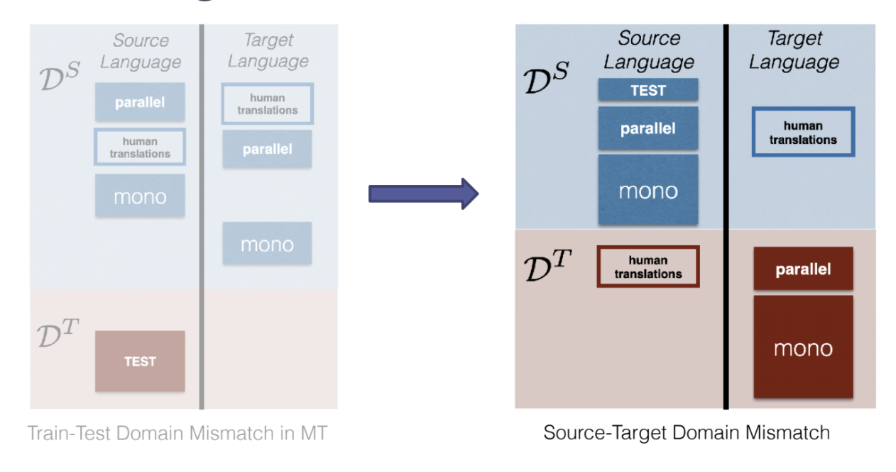
Figure 16: Source-Target Domain Mismatch in a Given Language

How to quantify STDM?

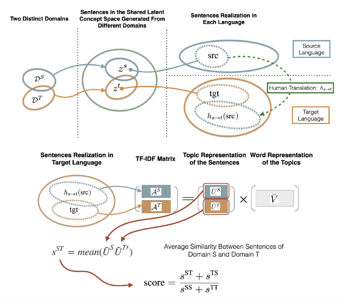
Figure 17: Quantifying STDM

In conclusion:

• STDM: a new kind of domain mismatch, intrinsic to the MT task.
• STDM is particularly significant in low resource language pairs.
• Metric & controlled setting enable study and better understanding of STDM.
• Methods that leverage source side monolingual data are more robust to STDM.
• In practice, the influence of STDM depends on several factors, such as the amount of parallel and monolingual data, the domains, language pair, etc. In particular, if domains are not too distinct, STDM may even help regularizing!