Generative Models

Autoencoders (AE)

Autoencoders are artificial neural networks trained in an unsupervised fashion that aim to learn representation of input data and then generate the data from the learned encoded representations. Autoencoders can be considered a special case of Amortized Inference where instead of finding the optimal latent to produce appropriate reconstruction of the input, we simply feed the output of encoder to decoder.

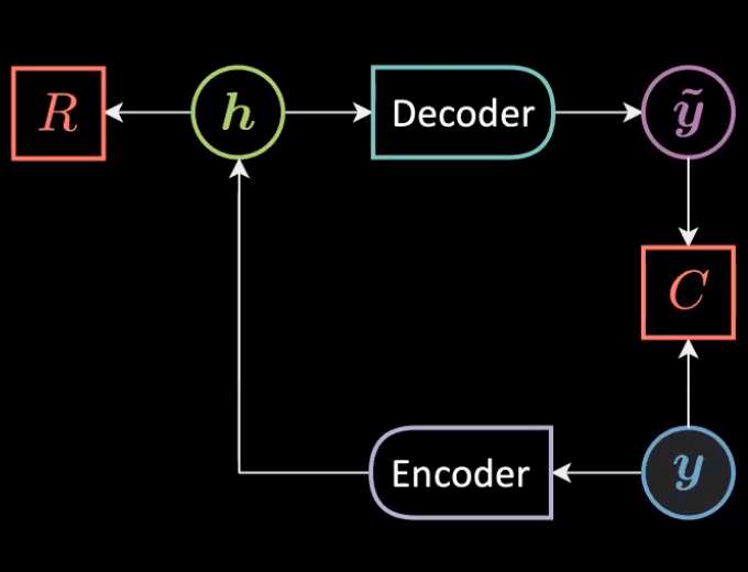
Fig. 1: General Architecture of an Autoencoder

We can express the above architecture mathematically as

With following dimensionalities:

The data is represented only through $\vy$ as the aim is to reconstruct the data that lives on the manifold (instance of unconditional EBM) through following energy function:

Under/Over Complete Autoencoder

In an autoencoder, when the dimension of hidden representation $d$, ($30$) is less than that of input size, $n$ ($784$), it can be referred as Under Complete Autoencoder.

Correspondingly, when the dimensionality of hidden representation, $d$ is greater than input dimensions $n$, it is said to be Over Complete Autoencoder.

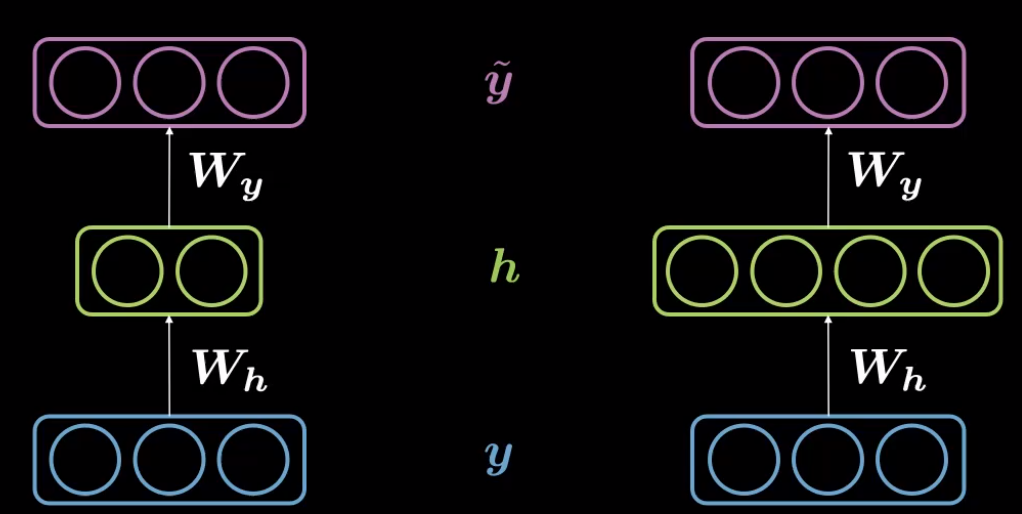
Fig. 2: Under Complete (left) and Over-Complete Autoencoder (right)

We are working with MNIST $28 \times 28$ images such that the transformation routine is defined from $784 (=28 \times 28) \rightarrow 30$ under the encoder followed by decoder that maps $30 \rightarrow 784$. The images are normalized and pixel values $\in [-1,1]$

class Autoencoder(nn.Module):
    def __init__(self):
        super().__init__()
        self.encoder = nn.Sequential(
            nn.Linear(28 * 28, d),
            nn.Tanh(),
        )
        self.decoder = nn.Sequential(
            nn.Linear(d, 28 * 28), # Rotation
            nn.Tanh(), # Squashing
        )

    def forward(self, y):
        h = self.encoder(y) # 784 -> 30
        y_tilde = self.decoder(h) # 30 -> 784
        return y_tilde

model = Autoencoder()
criterion = nn.MSELoss()

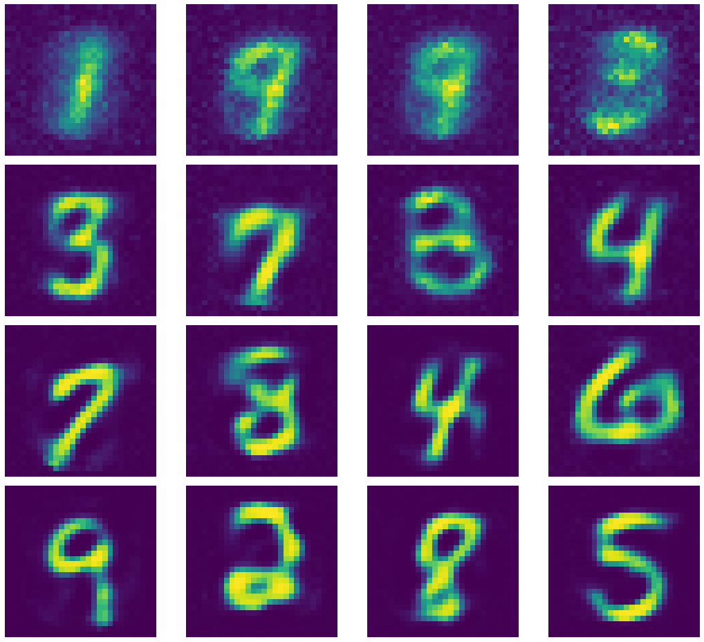
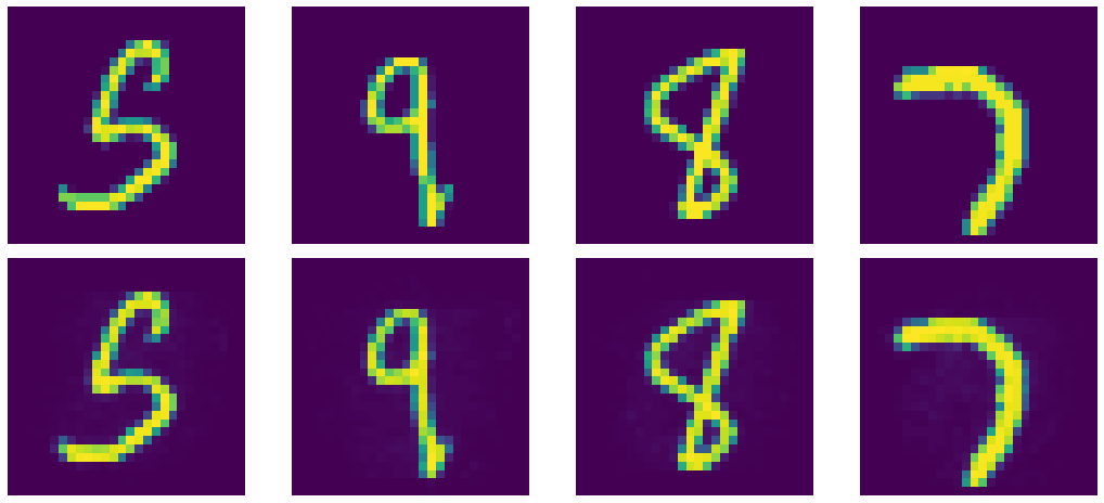
Fig. 3: Output Generated by Under Complete Autoencoder.

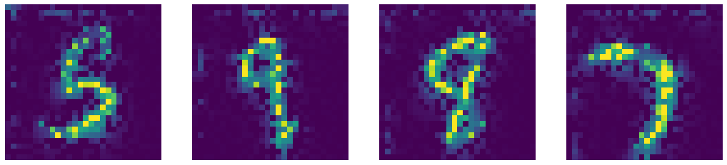
Let’s have a look on some of the kernels of the encoder.

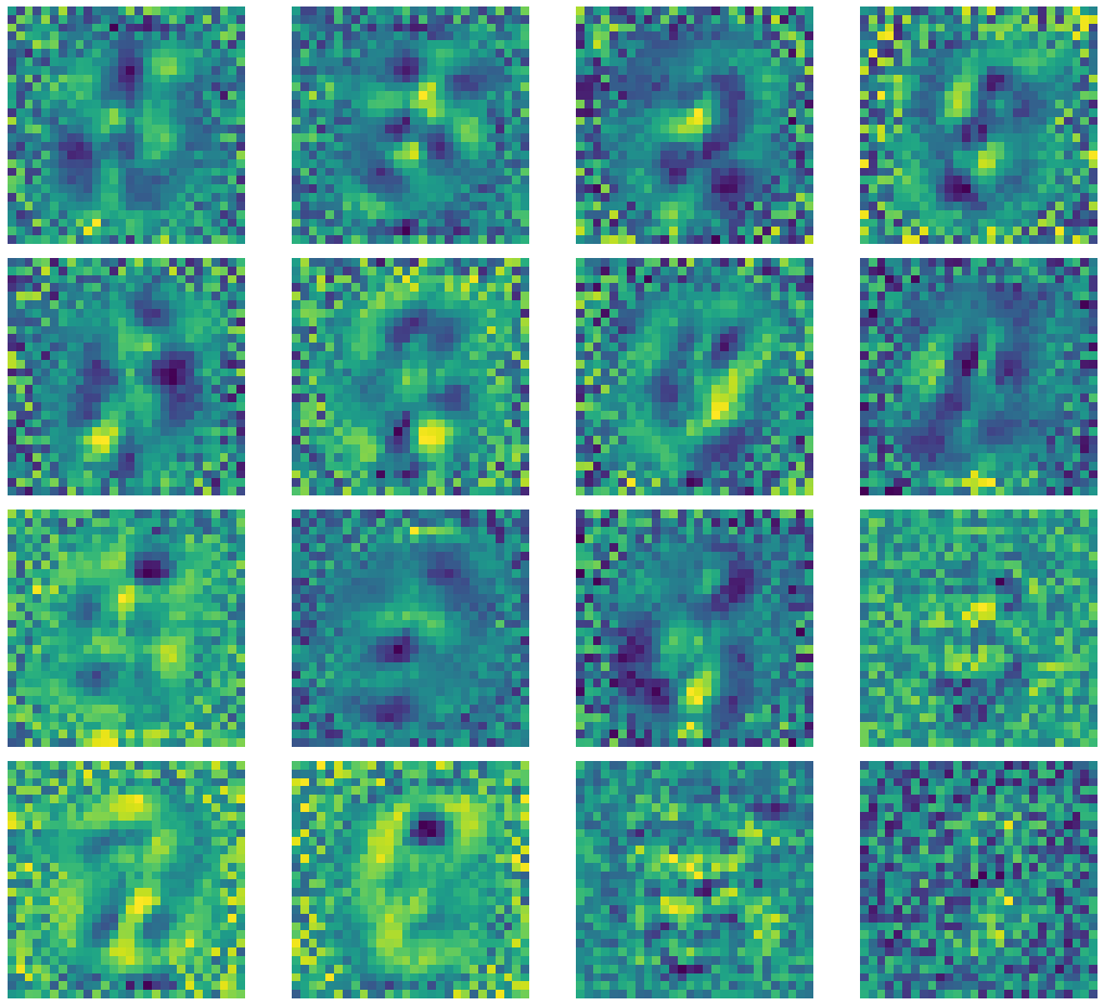
Fig. 4: Kernel Outputs of Under Complete Autoencoder.

If you notice there appears salt and pepper noise surrounding the center of images. This is due to the low spatial frequency along the region in the input image. The $+1$s and $-1$s in the noise cancel out to $0$, resulting in their average contribution as $0$. High-frequency regions appear around the central region as the digits in MNIST images are centered. The kernels with only noise indicate that the corresponding kernel collapsed or died.

Denoising Autoencoder (DAE)

In Denoising Autoencoder, we take a sample from dataset, inject some noise such the autoencoder is forced to reproduce the original sample. Therefore, the aim is to learn the vector field that should transform corrupted sample back to denoised part. Here, we set $d=500$ which is greater than number of pixels actually utilized to represent the digits in images. (Over Complete AE)

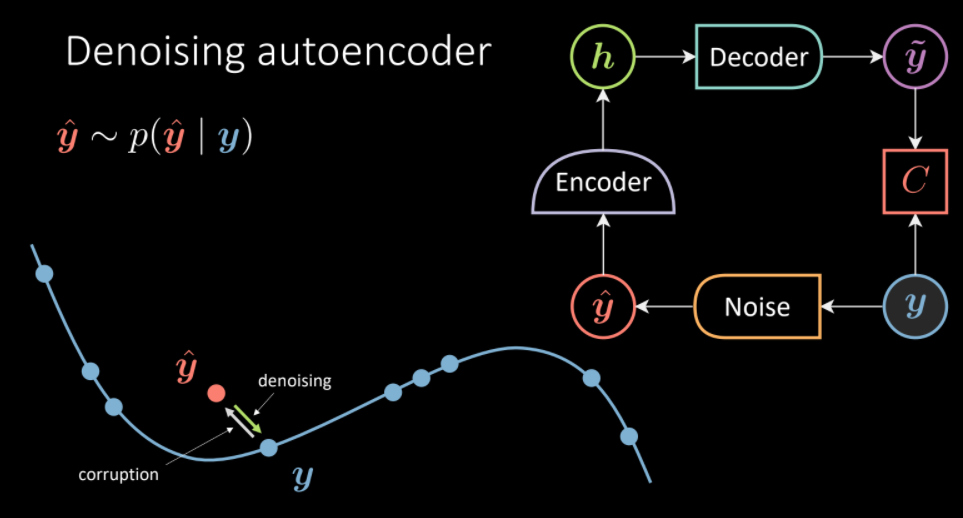
Fig. 5: Denoising Autoencoder Architecture. (Intution on left, transform corrupted $\vyhat$ towards the data manifold of $\vy$)

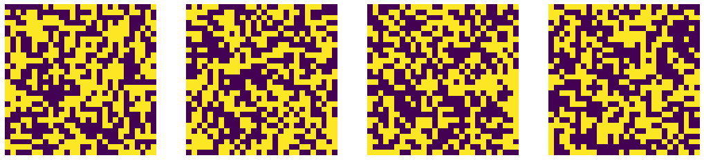
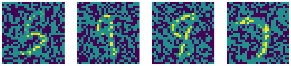
For the purpose of adding noise we perform the following steps:

1. Employ do=nn.Dropout() to randomly turn neuron off i.e. some pixel values will result in 0. (Original image is composed of pixel values $[-1,1]$)
2. Create a noise mask using the dropout do(torch.ones(img.shape))
3. Generate corrupted image by multiplying the original image with noise mask. img_bad=(img*noise)

The criterion for the model stay same i.e. to reproduce original sample given a noisy sample.

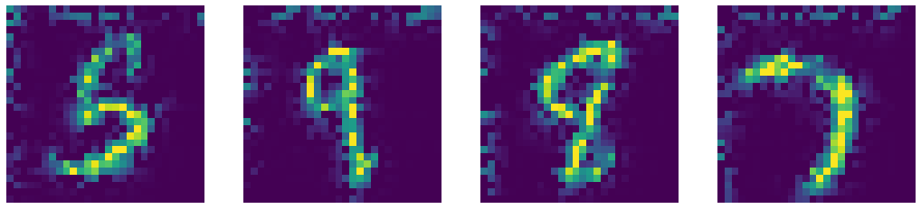
Again, let’s have a look at the kernels of the encoder. As you can see there is no salt and pepper noise as the surrounding region is no longer zero-mean and the kernel is forced to learn to ignore the region out of interest.

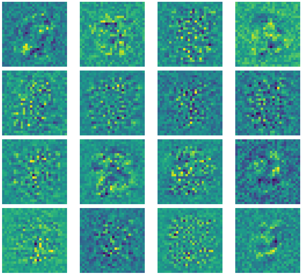
Fig. 6: Kernels of Denoising Autoencoder.

Comparing our denoised autoencoder with Computer Vision Inpainting methods such as Telea and Navier-Stokes methods.

Noise
Noised Input
Denoised Output by DAE
Telea Inpainting Output
Naiver-Stoke Inpainting Output
Fig. 7: Comparison of outputs of Denoised Autoencoder and state-of-the-art Computer Vision Inpainting algorithms.

Recall that an Denoised Autoencoder is an Constrastive EBM that assigns low-energy to samples lying on the actual data manifold (observed during training). Now, to test this out we merge two digits (perform alpha composite) and pass through the autoencoder:

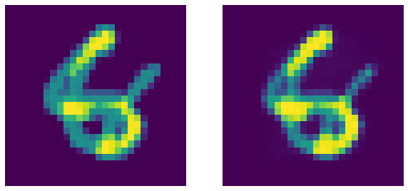
Fig. 8: Garbage (merged digits) on left and corresponding DAE's output. DAE as expected fails to denoise the image (this is a good thing!).

Interestingly, the autoencoder fails to reconstruct the merged garbage input as it was not observed during training. Therefore, the autoencoder can be used to estimate how noisy a given input sample is.

Variational Autoencoder (VAE)

Varitational Autoencoders are type of generative models, where we aim to represent latent attribute for given input as a probability distribution. The encoder produces $\vmu$ and $\vv$ such that a sampler samples a latent input $\vz$ from these encoder outputs. The latent input $\vz$ is simply fed to encoder to produce $\vyhat$ as reconstruction of $\vy$.

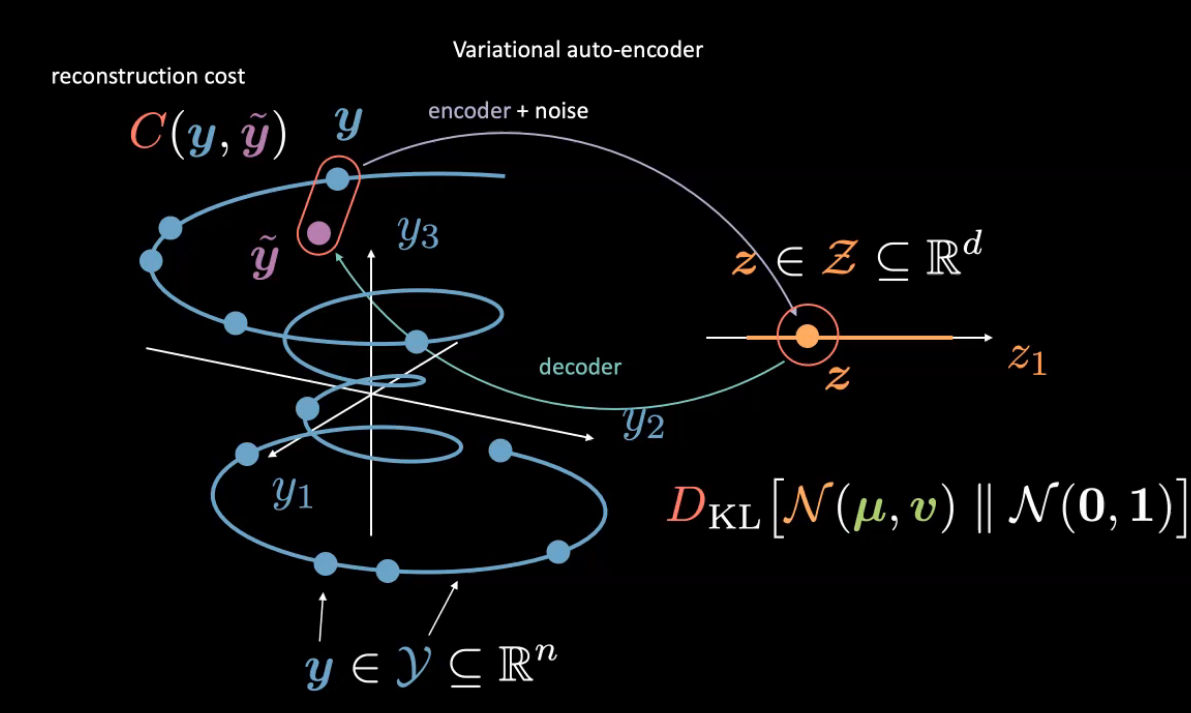
Fig. 9: Variational Autoencoder Intution

Here, we consider the latent random variable as $\vz$ belonging to a Gaussian with mean $\vmu$ and variance $\vy$. (Feel free to use any other distribution). Unlike before, we do not normalize the images.

Encoder and Decoder

The last layer of encoder has an output of dimension $2d$: first $d$ values refer to means, $\vmu$ and remaining $d$ values are variances $\vv$. The decoder has a sigmoid activation for last layer to maintain output range $[0,1]$.

d = 20

class VAE(nn.Module):
    def __init__(self):
        super().__init__()

        self.encoder = nn.Sequential(
            nn.Linear(784, d ** 2),
            nn.ReLU(),
            nn.Linear(d ** 2, d * 2)
        )

        self.decoder = nn.Sequential(
            nn.Linear(d, d ** 2),
            nn.ReLU(),
            nn.Linear(d ** 2, 784),
            nn.Sigmoid(),
        )

Reparameterise and forward function

During training, the reparameterise function is used for the reparameterisation trick: We cannot backpropagate through the sampler, we simply compute $\vz=\vmu+\epsilon\odot\sqrt{\vv}$ where $\epsilon \in \orange{\mathcal{N}}(0,\mathbb{I}_d)$. This allows to flow gradient back to encoder. During test time, we simply use $\vmu$

def reparameterise(self, mu, logvar):
    if self.training:
        std = logvar.mul(0.5).exp_()
        epsilon = std.data.new(std.size()).normal_()
        return eps.mul(std).add_(mu)
    else:
        return mu

def forward(self, x):
    mu_logvar = self.encoder(x.view(-1, 784)).view(-1, 2, d)
    mu = mu_logvar[:, 0, :]
    logvar = mu_logvar[:, 1, :]
    z = self.reparameterise(mu, logvar)
    return self.decoder(z), mu, logvar

We use log variance instead of variance (change of scale) because we want to ensure

1. Variance is non-negative.
2. Full range of variance, to make training stable.

Recall the free energy for VAE,

To regularise the expressivity of the latent, we include KL-divergence between the Gaussian of latent variable and a Normal distribution ($\orange{\mathcal{N}}(0,1))$. (Also see Week 8-Practicum for bubble explanation of VAE loss)

Therefore, we define the loss function as

def loss_function(x_hat, x, mu, logvar, β=1):
    BCE = nn.functional.binary_cross_entropy(
        x_hat, x.view(-1, 784), reduction='sum'
    )
    KLD = 0.5 * torch.sum(logvar.exp() - logvar - 1 + mu.pow(2))

    return BCE + β * KLD

Since, VAE is a generative model, we sample from the distribution to generate the following digits:

N = 16
z = torch.rand((N,d))
sample = model.decoder(z)

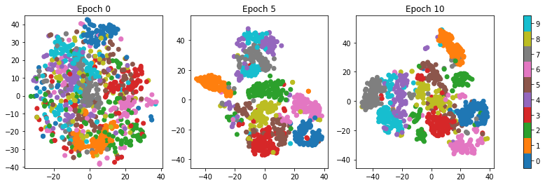
Fig. 10: TSNE visualization of samples generated through VAE.

The regions (classes) get segregated as the reconstruction term forces the latent space to get well defined. The data gets clustered into classes without actually using the labels.

Generative Adversarial Nets (GANs)

GANs have the same feel as DAE with some tweaks. DAE involves generating corrupt samples using the input and a distribution followed by denoising them using a decoder. GANs instead directly sample the distribution (without the input) to produce output $\vyhat$ using the Generator (or decoder in DAE terms). The input $\vy$ and $\vyhat$ are provided to the Cost network separately to measure incompatibility between them.

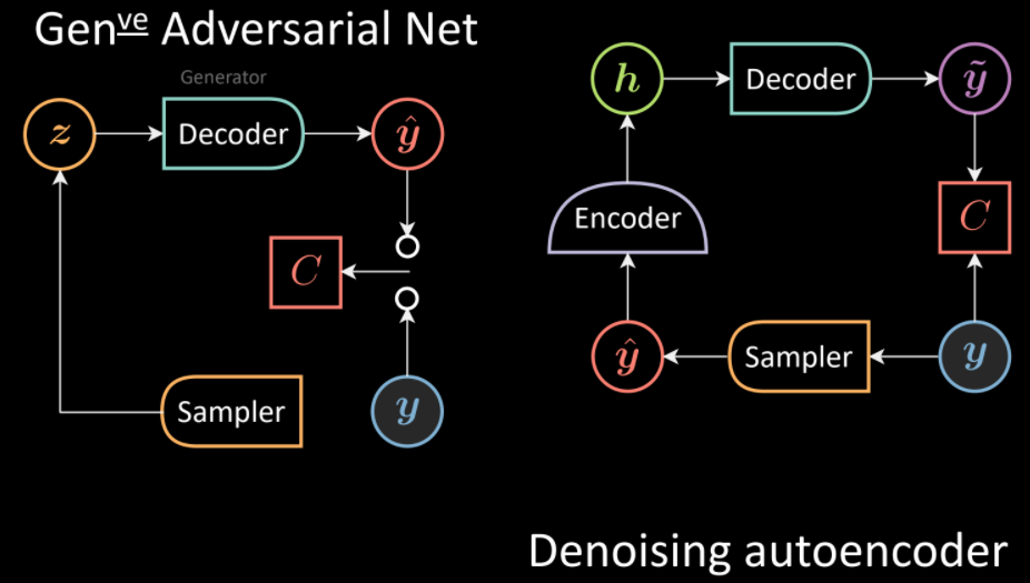
Fig. 11: Comparison of GANs (left) and DAE (right) architectures.

Similarly, we can extend the analogy with VAE. In contrast to VAE where the sampler is conditioned on the output of the encoder, in GANs there is an unconditioned sampler and again, decoder corresponds to Generator.

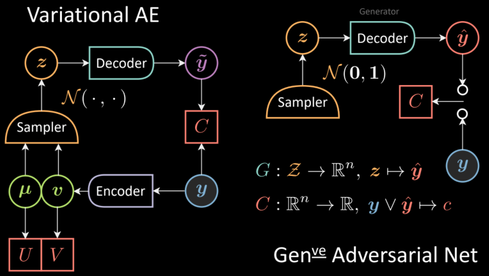
Fig. 12: Comparison of VAE(left) and GANs (right) architectures.

The Generator maps the latent space to data space:

The observed $\vy$ and $\vyhat$ are fed to a Cost network to measure incompatibility:

Training GANs

We define the loss functional for the Cost Network (Discriminator):

The aim is to push down sample of $\vy$ and push up the energy of $\vyhat$ upto $m$ (if $\red{C}\geq m$ no gradient is received as $\texttt{ReLU}(\cdot)$ would result the output to $0$).

For training the generator, the aim is to simply minimize the cost:

A possible choice of $\red{C}(\vy)$ can be

The cost network would push good samples to 0 and bad sample to energy level $m$. Using the above $\red{C}(\vy)$, there would exist a quadratic distance between the points on manifold, $\vy}$ and points generated by the generator $\vyhat$. During the training, generator is updated to try to produce samples that would gradually have low energy as $\vy$ guided by $\red{C}$. Once trained, the generator should produce samples near to data manifold.

Adopting another analogy , the generative model can be thought as team of counterfeiters, trying to produce fake currency. Their aim to produce fake currency which is indistinguishable from real currency. The discriminator can be viewed as police, trying to detect among counterfeit and fake currency bills. Gradients from backprop can be seen as spies that give opposite direction to counterfeiters (generator) in order to fool the police (discriminator).

Implementating Deep Convolutional Generative Adversarial Nets (DCGANs)

Follow this link for complete code.

The Generator upsamples the input using several nn.ConvTranspose2d modules to produce image from random vector nz (noise).

class Generator(nn.Module):
    def __init__(self, ngpu):
        super(Generator, self).__init__()
        self.ngpu = ngpu
        self.main = nn.Sequential(
            # input is Z, going into a convolution
            nn.ConvTranspose2d(     nz, ngf * 8, 4, 1, 0, bias=False),
            nn.BatchNorm2d(ngf * 8),
            nn.ReLU(True),
            # state size. (ngf*8) x 4 x 4
            nn.ConvTranspose2d(ngf * 8, ngf * 4, 4, 2, 1, bias=False),
            nn.BatchNorm2d(ngf * 4),
            nn.ReLU(True),
            # state size. (ngf*4) x 8 x 8
            nn.ConvTranspose2d(ngf * 4, ngf * 2, 4, 2, 1, bias=False),
            nn.BatchNorm2d(ngf * 2),
            nn.ReLU(True),
            # state size. (ngf*2) x 16 x 16
            nn.ConvTranspose2d(ngf * 2,     ngf, 4, 2, 1, bias=False),
            nn.BatchNorm2d(ngf),
            nn.ReLU(True),
            # state size. (ngf) x 32 x 32
            nn.ConvTranspose2d(    ngf,      nc, 4, 2, 1, bias=False),
            nn.Tanh()
            # state size. (nc) x 64 x 64
        )

    def forward(self, input):
        if input.is_cuda and self.ngpu > 1:
            output = nn.parallel.data_parallel(self.main, input, range(self.ngpu))
        else:
            output = self.main(input)
        return output

Discriminator is essentially a image classifier that uses nn.Sigmoid() to classify the input as real/fake.

class Discriminator(nn.Module):
    def __init__(self):
        super().__init__()
        self.main = nn.Sequential(
            # input is (nc) x 64 x 64
            nn.Conv2d(nc, ndf, 4, 2, 1, bias=False),
            nn.LeakyReLU(0.2, inplace=True),
            # state size. (ndf) x 32 x 32
            nn.Conv2d(ndf, ndf * 2, 4, 2, 1, bias=False),
            nn.BatchNorm2d(ndf * 2),
            nn.LeakyReLU(0.2, inplace=True),
            # state size. (ndf*2) x 16 x 16
            nn.Conv2d(ndf * 2, ndf * 4, 4, 2, 1, bias=False),
            nn.BatchNorm2d(ndf * 4),
            nn.LeakyReLU(0.2, inplace=True),
            # state size. (ndf*4) x 8 x 8
            nn.Conv2d(ndf * 4, ndf * 8, 4, 2, 1, bias=False),
            nn.BatchNorm2d(ndf * 8),
            nn.LeakyReLU(0.2, inplace=True),
            # state size. (ndf*8) x 4 x 4
            nn.Conv2d(ndf * 8, 1, 4, 1, 0, bias=False),
            nn.Sigmoid()
        )

    def forward(self, input):
        output = self.main(input)
        return output.view(-1, 1).squeeze(1)

We use Binary Cross Entropy to train the networks.

criterion = nn.BCELoss()

We have two optimizers for each network. (We want to push up the energy of bad (recognizable fake images) samples and push down energy of good samples (real looking images).

optimizerD = optim.Adam(netD.parameters(), lr=opt.lr, betas=(opt.beta1, 0.999))
optimizerG = optim.Adam(netG.parameters(), lr=opt.lr, betas=(opt.beta1, 0.999))

For training, we first train the discriminator with real images and labels stating the images being real. Followed by generator generating fake images from noise. The discriminator is again trained but this time with fake images and labels stating them as fake.

# This part is inside the training loop!
        # train with real
        netD.zero_grad()
        real_cpu = data[0]
        batch_size = real_cpu.size(0)
        label = torch.full((batch_size,), real_label,
                           dtype=real_cpu.dtype)

        output = netD(real_cpu)
        errD_real = criterion(output, label)
        errD_real.backward()
        D_x = output.mean().item()

        # train with fake
        noise = torch.randn(batch_size, nz, 1, 1,)
        fake = netG(noise)
        label.fill_(fake_label)
        output = netD(fake.detach())
        errD_fake = criterion(output, label)
        errD_fake.backward()
        D_G_z1 = output.mean().item()
        errD = errD_real + errD_fake
        optimizerD.step()

To train the generator, we compute the error by incompatibility between characteristics of real image and fake image as identified by the discriminator. Such that the generator can use this discrepancy measure to better fool the discriminator.

# This part is inside the training loop!
        netG.zero_grad()
        label.fill_(real_label)  # fake labels are real for generator cost
        output = netD(fake)
        errG = criterion(output, label)
        errG.backward()
        D_G_z2 = output.mean().item()
        optimizerG.step()