Low Resource Machine Translation I

Neural Machine Translation (NMT)

Neural Machine Translation (NMT) is an end-to-end learning approach for automated translation, with the potential to overcome many of the weaknesses of conventional phrase-based translation systems. Its architecture typically consists of two parts, one to consume the input text sequence (encoder) and one to generate translated output text (decoder). NMT is often accompanied by an attention mechanism which helps it cope effectively with long input sequences. The decoder learns to (soft) align via attention. A translation example from Italian to English is shown in the figure below:

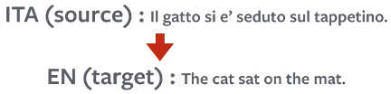
Figure 1: A translation example from Italian to English

Parallel Dataset

A parallel dataset contains a collection of original texts in language L1 and their translations into languages L2 (or consist of texts of more than two languages). As shown in the figure below, it can be used as labelled data to train NMT systems.

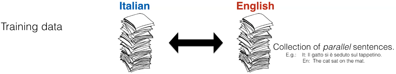
Figure 2: A parallel dataset consist of Italian and English

Train NMT

The standard way of training NMT is by using maximum likelihood. Give a source sentence $\vx$ and the model parameters $\vtheta$, we will seek to maximize the log likelihood of the joint probability of all the ordered sequence of tokens in the target sentence $\vy$, as illustrated by the equation below:

It is used as a score to indicate how likely the target sentence actually to be a translation from the source sentence. A minus sign is added in front of the equation to turn this into a minimization problem.

Language Model

In language modelling, given a token $\vx_t$ at time $t$, we are trying to predict the next word $\vy_t$. As shown in the figure below, hidden state $\vz_t$ is generated by a RNN/CNN/Transformer block depending on the input vector $\vx_t$ and the previous hidden state $\vz_{t-1}$.

Figure 3: Language Model

Encoder-Decoder Architecture (Seq2Seq)

Given a parallel dataset (with source sentences and target sentences), we can make use of the source sentences to train a seq2seq model.

Step 1: Represent source Represent each word in the source sentence as embeddings via source encoder.

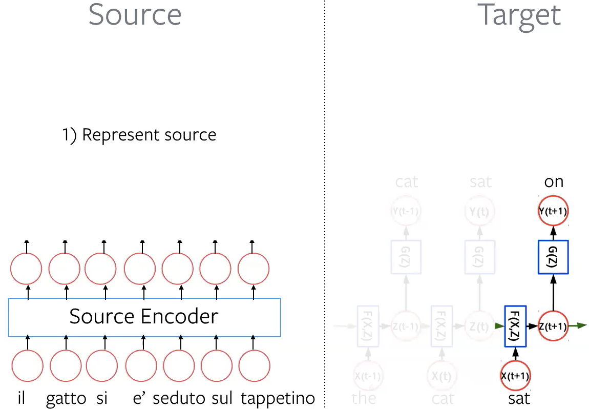
Figure 4: Represent source

Step 2: Score each source word (attention) Take the dot product between target hidden representation $\vz_{t+1}$ and all the embeddings from source sentence. Then use softmax to get a distribution over source tokens (attention).

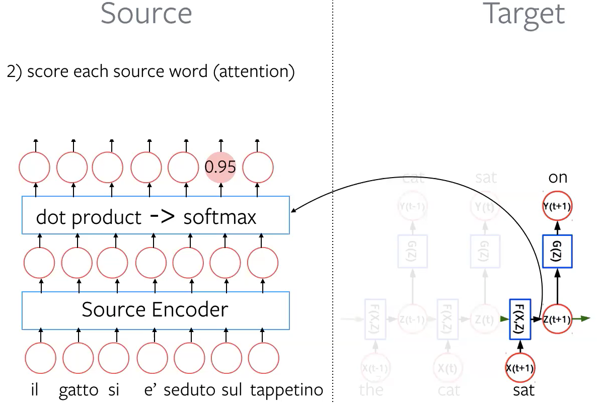
Figure 5: Score each source word

Step 3: Combine target hidden with source vector Take weighted sum (weights are in the attention score vector) of the source embeddings and combine it with target hidden representation $\vz_{t+1}$. After final transformation $G(\vz)$, we get a distribution $\vy_{t+1}$ over the next word.

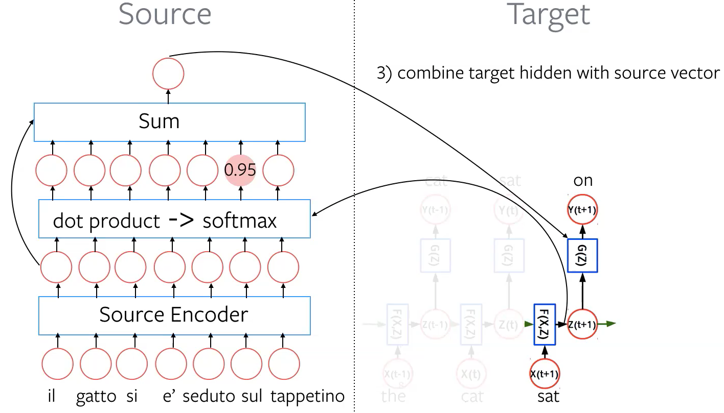
Figure 6: Combine target hidden with source vector

Alignment is learnt implicitly in seq2seq model. All tokens can be processed in parallel efficiently with CNNs or Transformers.

Test NMT

After we have the translation model, and know how good they are doing on the training set, we will want to test to see how the model will actually generate translations from the source sentences.

Beam Decoding is used to search in the space of $\vy$ according to

Each potential choice (the number of words in vocabulary) has a probability score. At every step, beam search selects the top $k$ scoring among all the branches (maintain a queue with $k$ top scoring paths), then expand each of them and retain the top $k$ scoring paths. As illustrated by the example below:

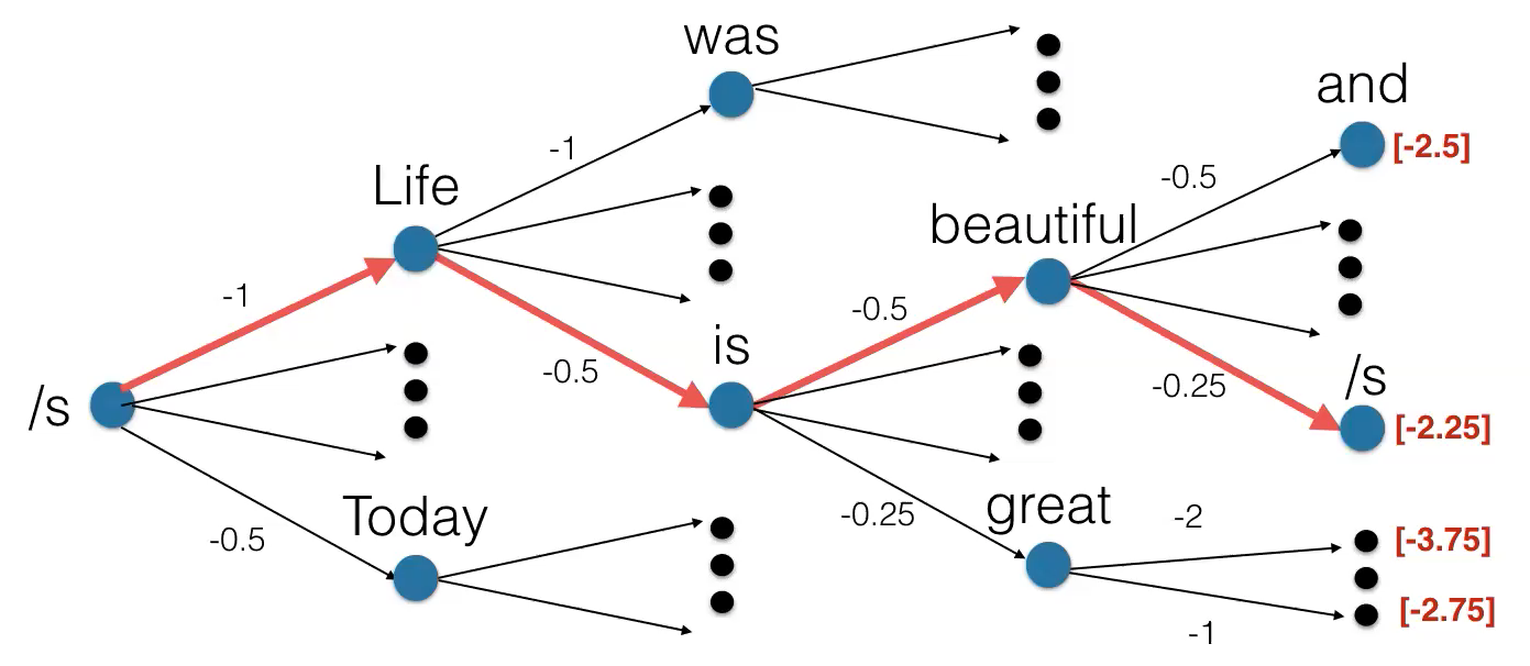
Figure 7: Beam Search

Let $k = 2$

1. Start from symbol /s, pick the top 2 scoring from all the possible choices (Life, Today)
2. Continue from Life and Today, expand each of them and calculate the path score back to the start symbol, pick the top 2 scoring path (“Like was” and “Like is”)
3. So on and so for, keep proceeding until hit the end of the sentence
4. At the very last step, select the highest scoring path

Beam search is a greedy procedure and it is very effective in practice. There is a trade-off between computational cost and approximation error (the larger the value of $k$, the better the approximation and the higher the computational cost).

Issues of Beam Search: Beam search will always select the highest scoring path. Thus, the solution will be biased because of such strategy. It doesn’t handle uncertainty well.

Other decoding methods: sampling, top-$k$ sampling, generative and discriminative reranking

NMT Training & Inference Summary

Training: predict one target token at the time and minimize cross-entropy loss

Inference: find the most likely target sentence (approximately) using beam search

Evaluation: compute BLEU on hypothesis returned by the inference procedure

We first compute the geometric average of the modified n-gram precisions, $p_n$

Candidate translations longer than their references are already penalized by the modified n-gram precision measure: there is no need to penalize them again. Consequently, we introduce a multiplicative brevity penalty factor, BP (denoted as \(f_{\text{BP}}\) in the formula). With BP in place, a high-scoring candidate translation must now match the reference translations in length, in word choice, and in word order.

In brief, BLEU score (denoted as $s_{\text{BLEU}}$ in the formula) measures the similarity between the translation generated by the model and a reference translation created by a human.

Machine Translation in Other Languages

The above theory has 2 assumptions:

1. The languages that we considered are English and Italian, both of which are European languages with some commonality.
2. We have a lot of data because, in general, we need three data points to estimate a parameter and these models have hundreds of millions of parameters.

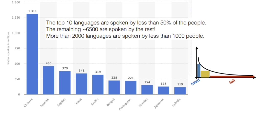
Figure 8: Statistics of the languages spoken in the world, tail represents the huge number of languages with not much speakers

If we consider the statistics, there are more than 6000 languages in the world and not more than 5% of the world population speaks native English. There are a number of languages for which we don’t have much data available and Google Translate performs poorly. The other issue with these languages is that they are mostly spoken and not written.

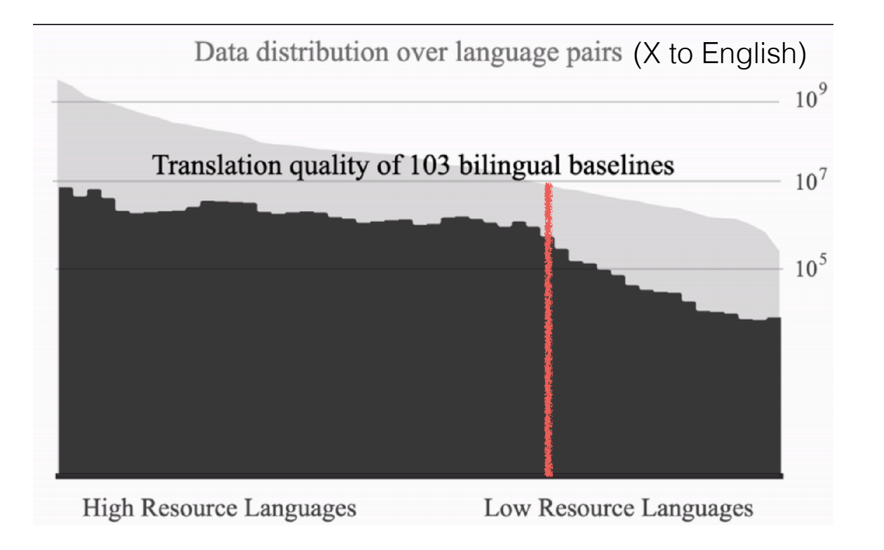
Figure 9: Translation quality degrades rapidly for low resource languages

Machine Translation in Practice

Let’s consider an English to Nepali Machine Translation system where we translate English news to Nepali. Nepali is a low resource language and the amount of parallel data for training is very small.

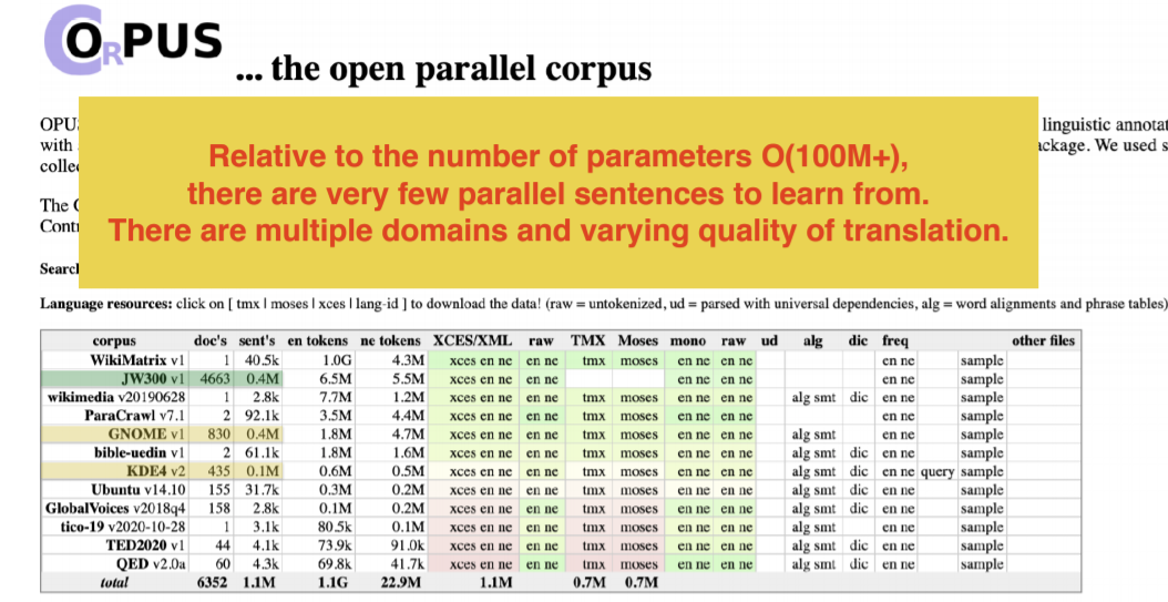
Figure 10: Open Parallel Corpus Dataset resources for English to Nepali

The open parallel corpus is a place where we can get these datasets. There are 2 issues here:

1. Now, if we look for Nepali dataset, we see that either there is very less amount of quality data set or huge dataset with no useful content.
2. There are possibilities that the source and target data are not parallel. We might have more data in English in some categories, more data in Nepali in other categories. There are cases these two don’t match.

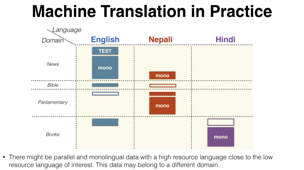
Figure 11: Machine Translation from English to Nepali with the help of other languages like Hindi

One way to solve these issues is to make use of other languages related to Nepali. For example, Hindi is a much higher resource language and belongs to the same family as Nepali. We can extend this to other languages also.

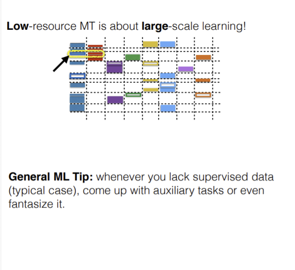
Low Resource Machine Translation

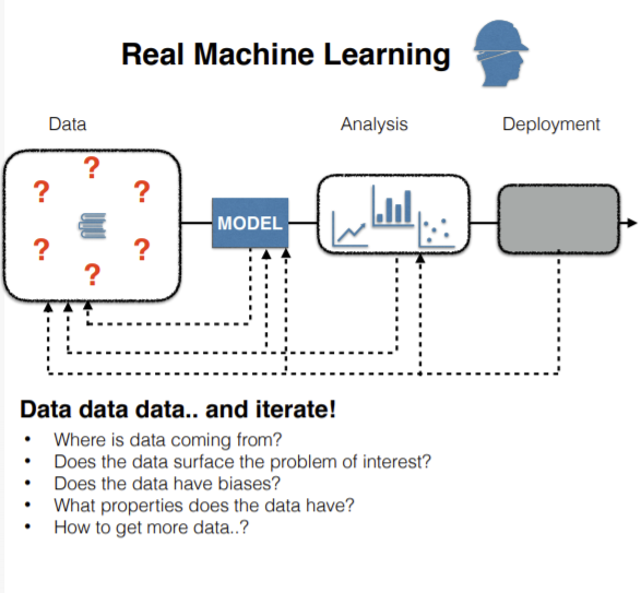
In practice, whenever a model is being trained, there is a lot of effort that goes in analyzing the model and the properties of the data. This whole thing is an iterative process and the machine learning practitioner needs to view this with a complete picture. Secondly, if there is less data, we can downscale the model, which isn’t desirable. We need to come up with ways to enlarge the dataset somehow or use unsupervised techniques.

(a) Data collection in ML	(b) Low-resource tasks in ML

Challenges

Loose definition of Low Resource MT: A language pair can be considered low resource when the number of parallel sentences is in the order of 10,000 or less.

Challenges encountered in Low Resource Machine Translation tasks:

• Datasets
  • Sourcing data to train on
  • High quality evaluation datasets
• Metrics
  • Human evaluation
  • Automatic evaluation
• Modeling
  • Learning paradigm
  • Domain adaption
  • Generalization
• Scaling

Additionally, there will be challenges that are encountered in general Machine Translation tasks:

• Exposure bias (training for generation)
• Modeling uncertainty
• Automatic evaluation
• Budget computation
• Modeling the tails
• Efficiency

MAD Cycle of Research

There are 3 pillars in the cycle of research:

1. Data: We collect data that we want to explore.
2. Model: We feed the collected data and use the data distribution, develop algorithms and build models.
3. Analysis: After we get the model, we test the model by checking how well it fits with the data distribution or how well it performs using different metrics.

This process is iterated several times to get a good a performance.

Figure 14: 3 Pillars in the cycle of research

The highlighted examples in the Figure 14 will be discussed more in detail in the following sections.

Data

Going back to the same example of English-Nepali news translation, we collect data belonging to different domains. Here, dataset of Bible and GNOME, Ubuntu won’t be of much help for news translation.

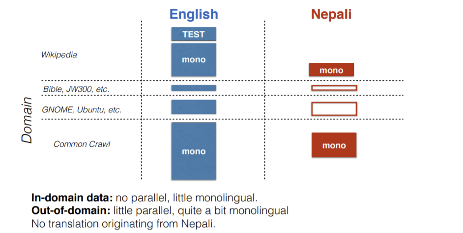
Figure 15: English-Nepali dataset

The question here is how can we evaluate the part of dataset that is not there on the right side (Nepali)? This lead to creation of FLoRes Evaluation Benchmark. It contains texts (taken from Wikipedia documents) from Nepali, Sinhala, Khmer, Pashto.

Note: These are not parallel dataset

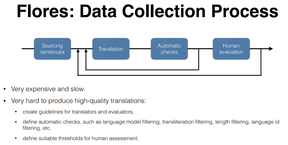
Figure 16: Flores Data Collection Process

These sentences are translated and the quality of the translations are determined using the automatic checks and human evaluation. There are several techniques in automatic checks, a model was trained on each language and perplexity was measured. If the perplexity is too high, then we go back to translation stage as shown above. Other checks are transliteration, using Google Translate, etc. There is no criteria or conditions for when this loop is stopped, essentially it depends on the perplexity and any outliers.

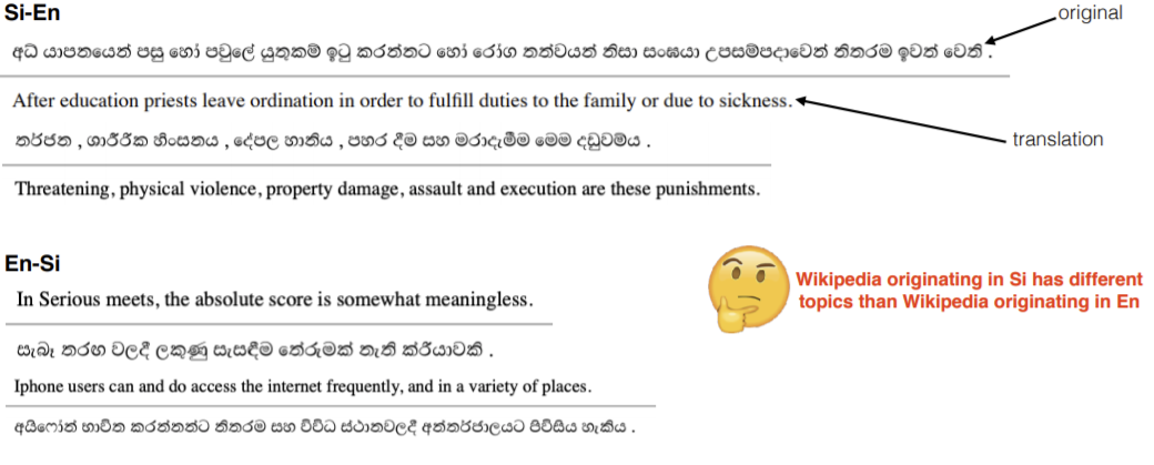
Figure 17: Some examples of English Sinhala translations

Figure 17 shows some examples. As we can see, they are not really fluent. One more issue with these is that the wikipedia articles of Sinhala language mostly contain topics of very limited number of domains (like their religion, country, etc.)