Joint Embedding Methods - Regularised

Non-Contrastive methods

Non-Contrastive methods and information theory:

Most of the non-contrastive methods are based on information theory. For example: Redundancy reduction ( Barlow Twins ) and Information. They don’t require special architectures or engineering techniques.

VicReg:

It tries to maximize the information content of the embeddings by producing embedding variables that are decorrelated to each other. If the variables are correlated to each other, they covariate together and the information content is reduced. Thus, it prevents an informational collapse in which the variables carry redundant information. Also, this method requires a comparatively small batch size.

Two types of collapse can occur in these architectures:
$\textbf{Type 1}:$ Irrespective of the input, the network generates the same representation
$\textbf{Type 2}:$ Special collapse - Although different images have different representations, the information content is really low in each representation.

Loss function:

The loss function is pushing:

1. Positive pairs closer - to be invariant to data augmentation
2. The variance of the embeddings large by pushing all of the diagonal terms of the covariance matrix large - to prevent the first kind of collapse
3. The covariance of the embeddings small by pushing all off the diagonal terms of the covariance matrix small- to prevent the second kind of collapse.

Clustering methods

SwAV

This method prevents trivial solution by quantizing the embedding space. SwAV does the following:

1. Generates representations and stack the generated representations ( into $\green{H_{x}}$ and $\green{H_{y}}$ ).
2. Applies sinkhorn clustering method to each of the stacked representation to generate corresponding clustered $\green{\boldsymbol{Q}}$ matrices where each row ( $\violet{q_{\vx}}$ ) represents a one hot vector indicating the cluster the corresponding representation belongs to
3. Performs second clustering for the representations $\vh_{\vx}$ and $\vh_{\vy}$ with soft-kmeans. This step generates predictions for $\green{q_{\vx}}$ and $\green{q_{\,\vy}}$, $\violet{\tilde{q_{\vx}}}$ and $\tilde{\violet{q_{\vy}}}$, from $\vh_{\vy}$ and $\vh_{\vx}$ respectively ( Thus, called swap prediction )
4. Minimizes the loss function which is the sum of two crossentropy functions between $\green{q_{\vx}}$ and $\violet{\tilde{q_{\vx}}}$ and $\green{q_{\vy}}$ and $\violet{\tilde{q_{\vy}}}$.

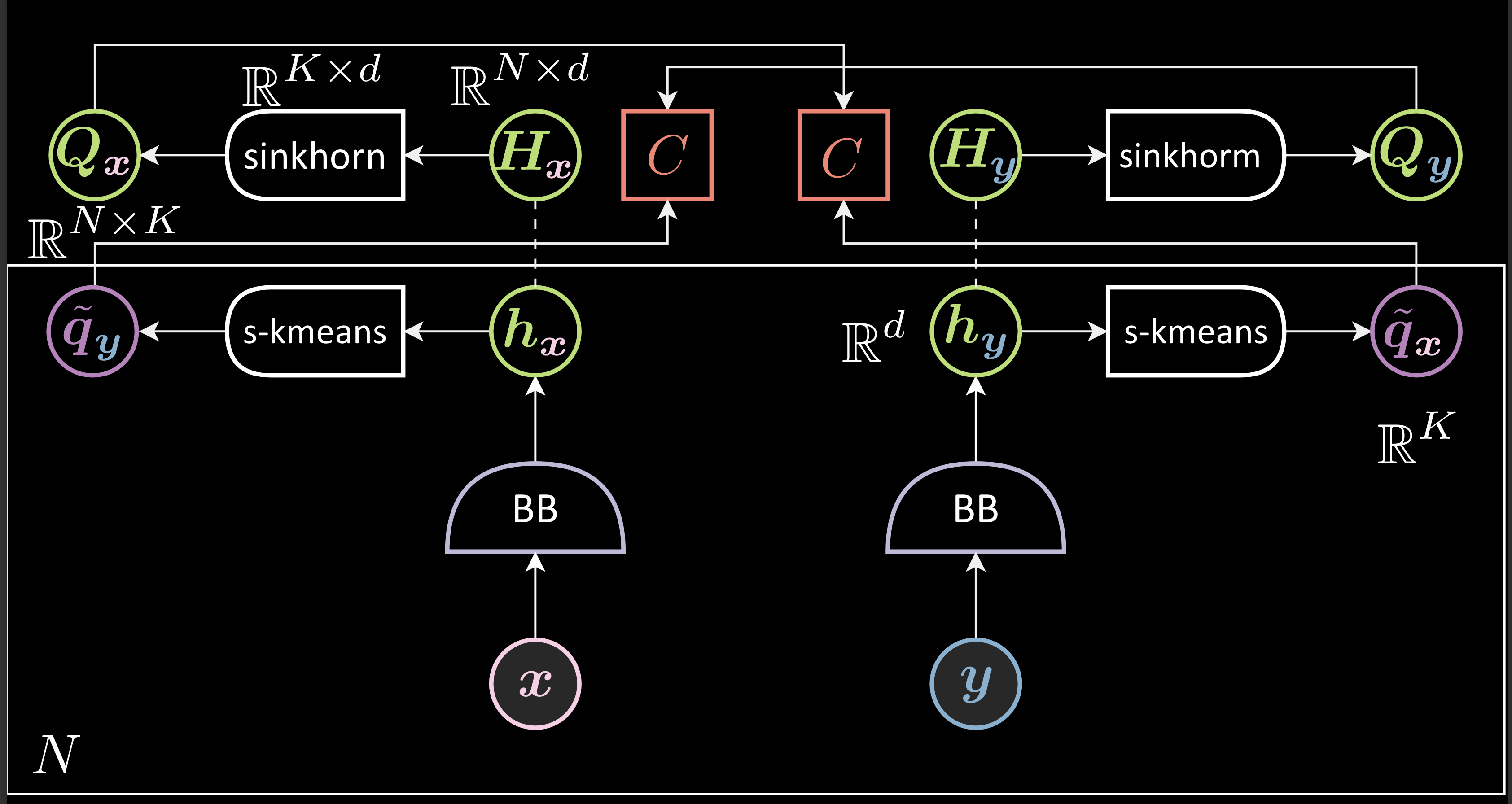
Fig. 8: SWaV

The Loss function:

Sinkhorn algorithm: Sinkhorn algorithm can distribute samples to not just one cluster but to every cluster. Thus, it can help us prevent all the data clustering into a single centroid or any such nonuniform distribution. It takes in hyperparameters that allow us to deploy different levels of uniform distribution across clusters degenerating to K-means algorithm on one extreme and to the perfectly uniform distribution on the other extreme

Softargmax clustering: Each $\green{h_{\vy}}$ is normalized. $\boldsymbol{W}\green{h_{\vy}}$ indicates similarity between $\green{h_{\vy}}$ and all other centroids. Softargmax turns the cosine similarly ( positive or negative ) into a probability.

Since this is predicting the $\green{q_{\vx}}$, we will compare the cross entropy of the prediction, $\violet{\tilde{q_{\vx}}}$, with the actual $\green{q_{\vx}}$ to measure the prediction.

Interpretation of clusters:

This method partitions latent space into a few clusters automatically without labels and the hope is that these clusters will be related to the actual classes. Thus, later, we would just need a few labeled data samples to assign each cluster to the corresponding label under supervised learning.

Invariance to data augmentation:

Instead of pushing the pairs closer to each other, you push both the representations to be inside the same cluster.

Preventing trivial solution

In a trivial solution, all the representations will be the same and thus belong to the same centroid. However, with sinkhorn, different clusters have an equal number of samples, thus the representations can’t be put into one centroid, preventing a trivial solution.

Other methods

The loss function for all the previous methods including contrasting methods needs a batch or pool of negative samples, thus creating problems with distributed training. However, the loss functions of these methods are local. These methods perform well but an understanding of why they don’t collapse is not yet available. Probably there’s some implicit regularization happening in these networks to prevent them from converging to a trivial solution.

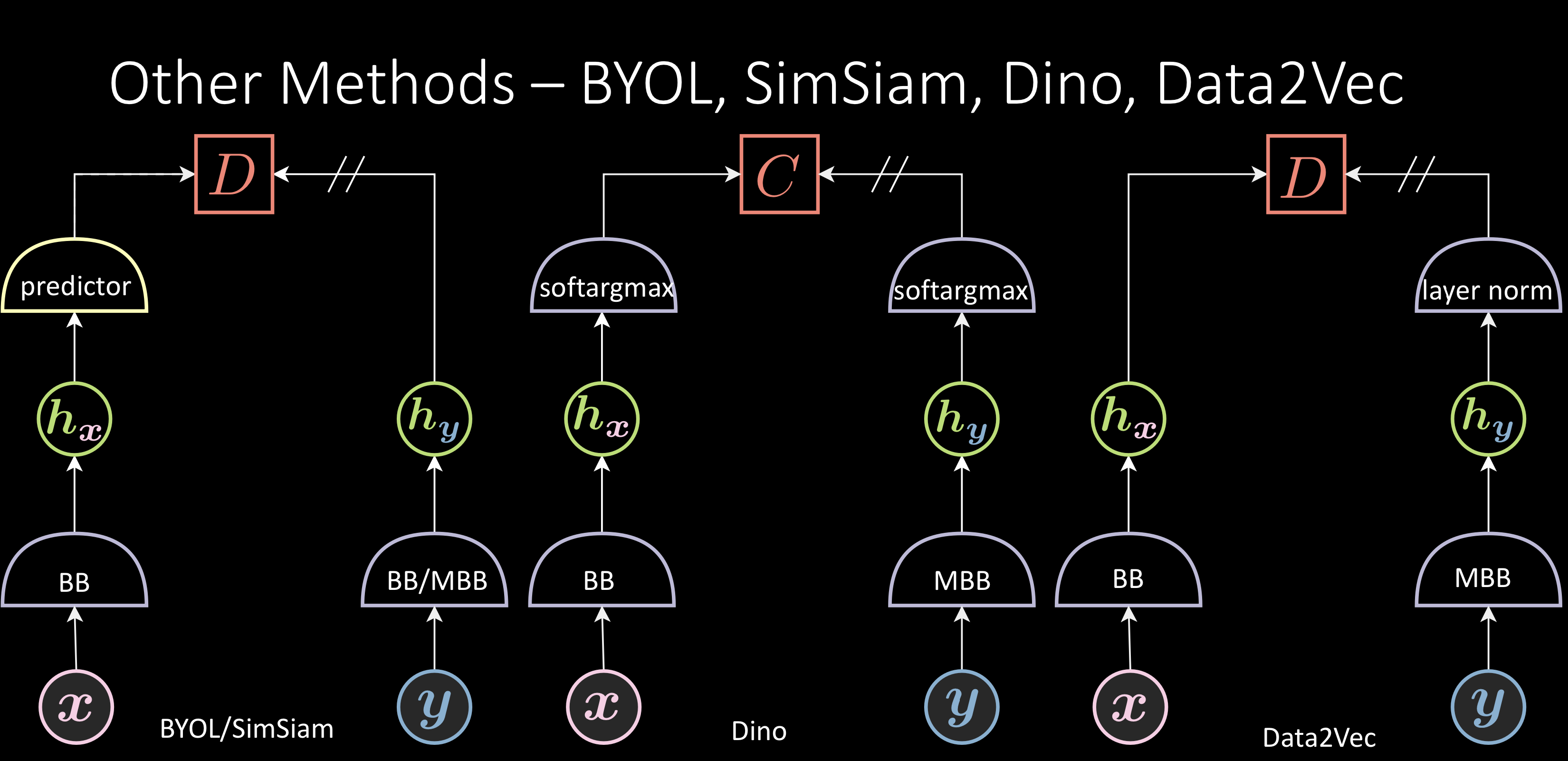
Fig. 10: Other Methods

BYOL:

BOYL adds a predictor, predicting $\green{h_{\vy}}$ from $\green{h_{\vx}}$. The energy function ( $\red{D}$ ) is a cosine similarity between $\green{h_{\vy}}$ and predicted $\green{h_{\vy}}$. There is no term for negative samples i.e., this method only pushes positive pairs closer and has no enforcement on negative pairs. It is thought that asymmetrical architecture with extra layers makes this method work.

SimSiam is a followup version that uses a regular backbone instead of the momentum backbone

Dino:

The two softargmax components used have different coldness or temperature. The energy function is the cross entropy between these two, pushing them together. Even this method doesn’t enforce anything on negative samples.

Data2Vec:

Adds a layer norm at the end of the representation.

Initialization of the network:

If you initialize the network with a trivial solution, then that network will never work. This is because if the trivial solution is already achieved, the loss function will produce a zero gradient and thus, can never escape from the trivial solution. However, in other cases, the training dynamic is adjusted in a way that they never converge in these methods.

Improvements for JEMs

We can further improve these models by experimenting with data augmentation and network architecture. We don’t have a good understanding of these but they are very important. In fact, finding good augmentation may boost more performance than changing the loss function.

Data Augmentation

Most dominant augmentations were proposed by simCLR and improved a little bit by BYOL:

1. Random Crop (the most critical one)
2. Flip
3. Color Jitter
4. Gaussian Blur

It has been found empirically that random crop is the most critical one. It might be because the random crop is the only we can change the spatial information about the images. Flip does the same partly but is weak. Color jitter and gaussian blur change channels.

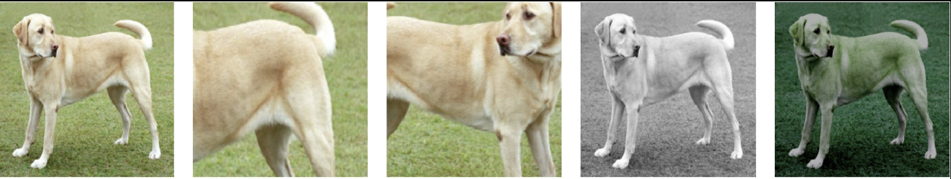
Fig. 5: Data Augmentation

Masking augmentation:

Recently people are moving towards masking augmentation instead of traditional augmentation in which we mask out most ( ~75% in the below image ) of the patches. It can replace random crop since it’s another way to remove the redundancy of the spatial information

Issues: This works well only with transformer type of architecture and not with convnet. This is because masking introduces too many random artificial edges. For any transformer, the first layer is the conv layer, with kernel size equal to the patch size and thus, this never experiences artificial edges. For convnets which have sliding windows, the artificial edges can’t be ignored and will result in noise.

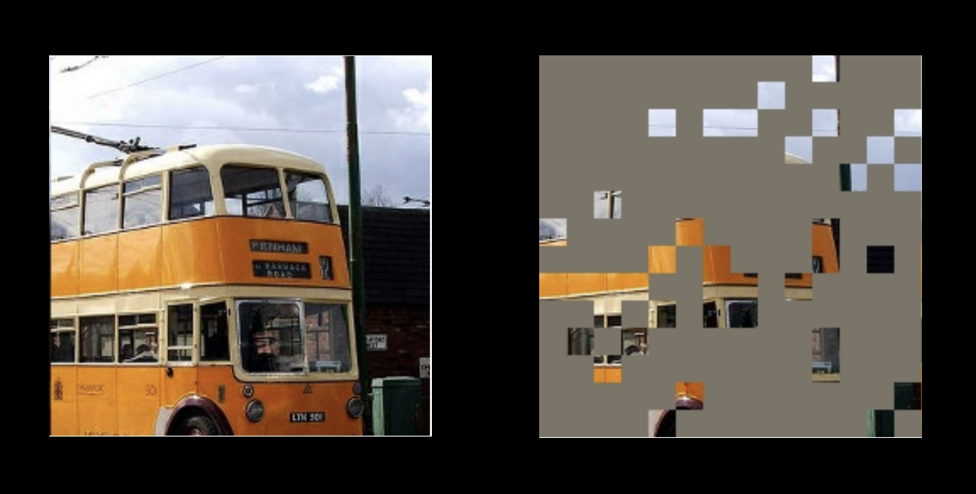
Fig. 6: Masked Augmentation

Network Architecture

Projector/Expander:

It is a two/three-layer feed-forward neural network and empirical results show that it is always better to add this in the network architecture.

The projector is used to project into a lower dimension and the expander is used to project into a higher dimension. A projector is used only during the pretraining and removed while performing the downstream task. This is because the projector removes a lot of information even if the output dimension of the projector and the backbone are the same.

Momentum Encoder:

Even without a memory bank, a momentum encoder usually helps the performance of the downstream tasks, especially with weak data augmentation.

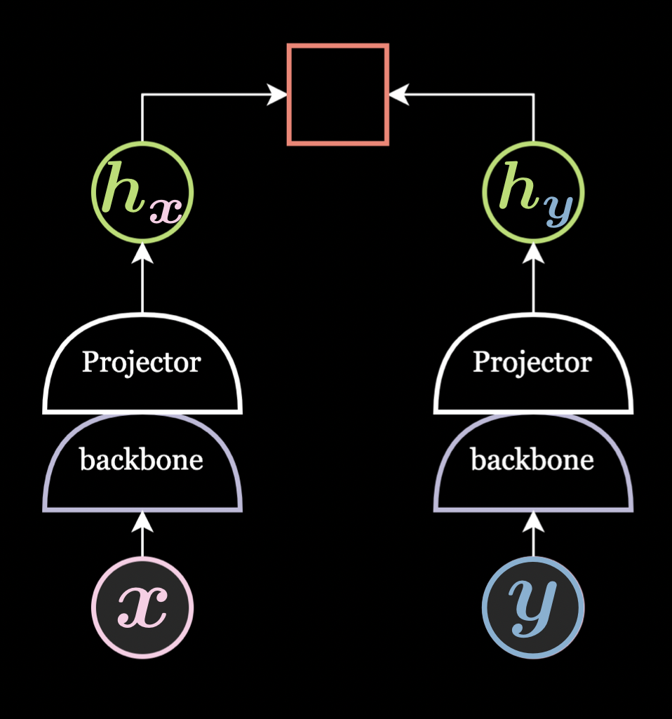
Fig. 7: Projector/Expander