MPC (EBM version)

Action plan

• Model predictive control [Here we are today]
  • Backprop through kinematic equation
  • Minimisation of the latent
• Truck backer-upper
  • Learning an emulator of the kinematics from observations
  • Training a policy
• PPUU
  • Stochastic environment
  • Uncertainty minimisation
  • Latent decoupling

State transition equations – Evolution of the state

Here we discuss a state transition equation where $\vx$ represents the state, $\vu$ represents control. We can formulate the state transition function in a continuous-time system where $\vx(t)$ is a function of continuous variable $t$.

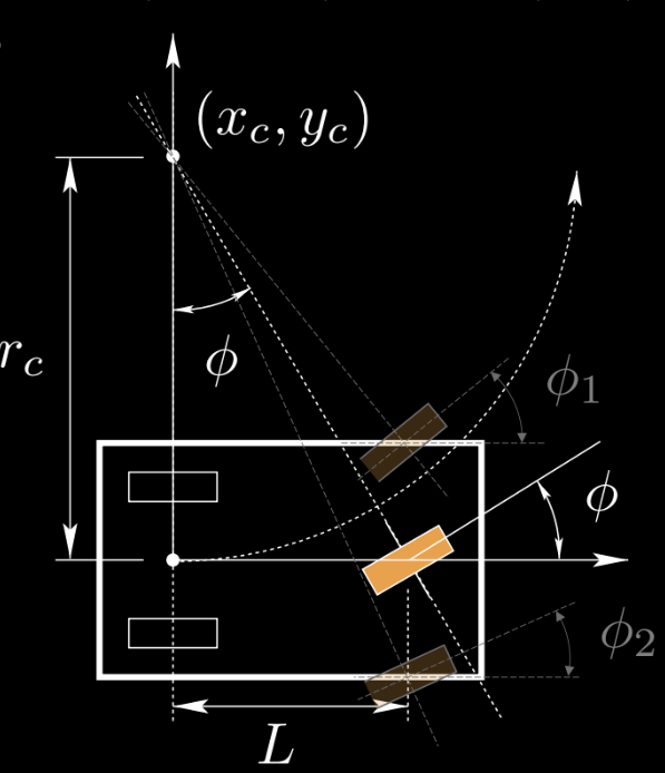
Figure 1: State and control illustration of a three-cycle

We use a tri-cycle as the example to study it. The orange wheel is the control $\vu$, $(x_c,y_c)$ is the instantaneous center of rotation. You can also have two wheels in the front. For simplicity, we use one wheel as the example.

In this example $\vx=(x,y,\theta,s)$ is the state, $\vu=(\phi,\alpha)$ is the control.

We can reformulate the differential equation from continuous-time system to discrete-time system

To be clear, we show the units of $\vx, \vu$.

Let’s take a look at different examples. We use different color for variables we care about.

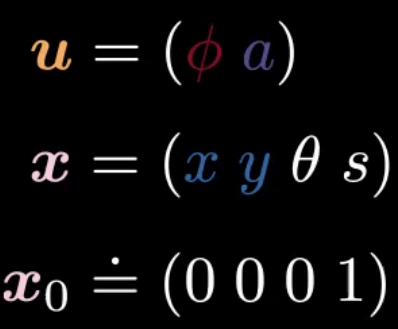
Figure 2: State Formulation

Example 1: Uniform Linear Motion: No acceleration, no steering

Figure 3: Control of Uniform Linear Motion

Figure 4: State of Uniform Linear Motion

Example 2: Crush into itself: Negative acceleration, no steering

Figure 5: Control of Curshing into itself

Figure 6: State of Curshing into itself

Example 3: Sine wave: Positive steering for the first part, negative steering for the second part

Figure 7: Control of Sine Wave

Figure 8: State of Sine Wave

Kelley-Bryson algorithm

What if we want the tri-cycle to reach a specified destination with a specified speed?

• This can be achieved by inference using Kelley-Bryson algorithm, which utilizes backprop through time and gradient descent.

Recap of RNN

We can compare the inference process here with the training process of RNN.

Below is an RNN schematic chart. We feed variable $\vx[t]$ and the previous state $\vh[t-1]$ into the predictor, while $\vh[0]$ is set to be zero. The predictor outputs the hidden representation $\vh[t]$.

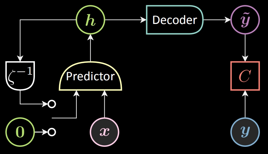
Figure 9: RNN schematic chart

Optimal control (inference)

In optimal control (inference) shown as below, we feed the latent variable (control) $\vz[t]$ and the previous state $\vx[t-1]$ into the predictor, while $\vx[0]$ is set to be $\vx_0$. The predictor outputs the state $\vx[t]$.

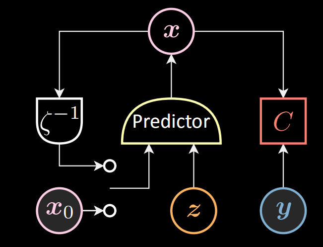
Figure 10: Optimal Control schematic chart

Backprop is implemented in both RNN and Optimal Control. However, gradient descent is implemented with respect to predictor’s parameters in RNN, and is implemented wrt latent variable $\vz$ in optimal control.

Unfolded version of optimal control

In unfolded version of optimal control, cost can be set to either the final step of the tri-cycle or every step of the tri-cycle. Besides, cost functions can take many forms, such as Average Distance, Softmin, etc.

Set the cost to the final step

From the figure below, we can see there is only one cost $c$ set in the final step (step 5), which measures the distance of our target $\vy$ and state $\vx[5]$ with control $\vz[5]$

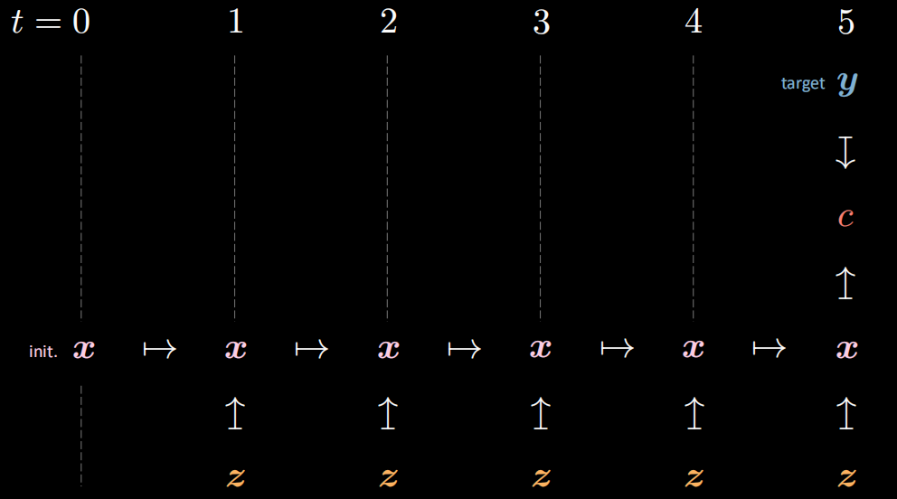
Figure 11: Cost to the final step

$(1)$ If the cost function only involves the final position with no restrictions on the final speed, we can obtain the results after inference shown as below.

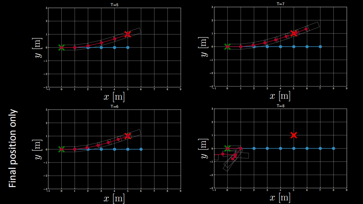
Figure 12: Cost function involving only the final position

From the figure above, it is seen that when $T=5$ or $T=6$, the final position meets the target position, but when $T$ is above 6 the final position does not.

$(2)$ If the cost function involves the final position and zero final speed, we can obtain the results after inference shown as below.

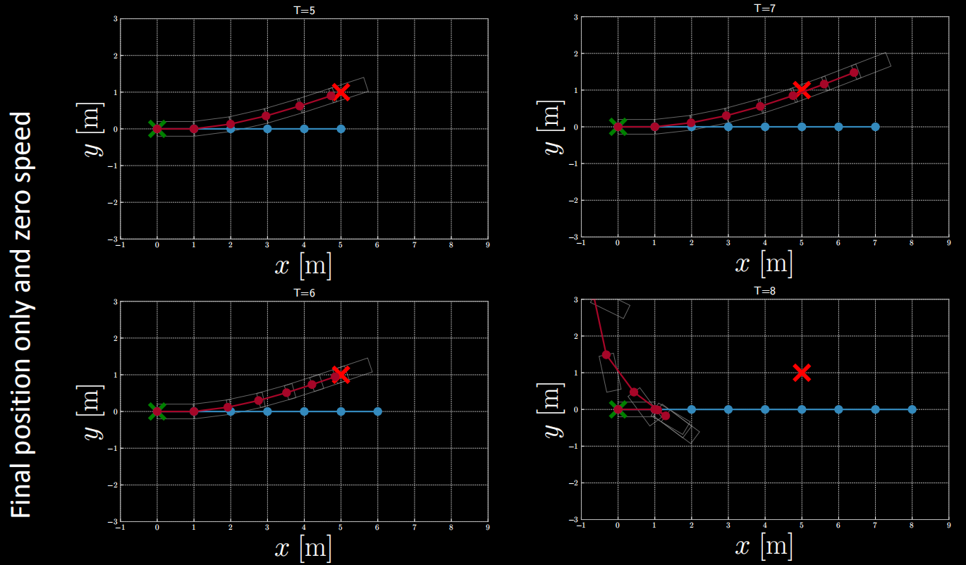
Figure 13: Cost function involving the final position and zero final speed

From the figure above, it is seen that when $T=5$ or $T=6$, the final position roughly meets the target position, but when $T$ is above 6 the final position does not.

Set the cost to every step

From the figure below, we can see there is a cost $c$ set in every step.

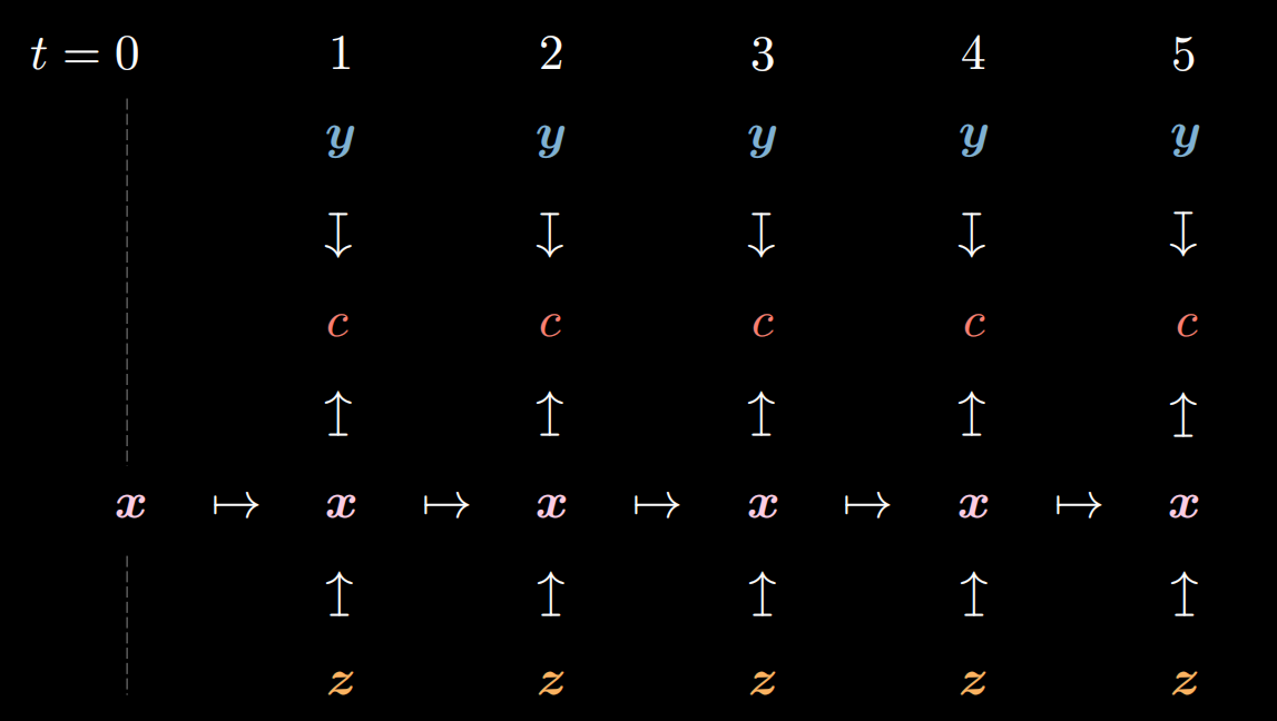
Figure 14: Cost to every step

$(1)$ Cost Example: Average Distance

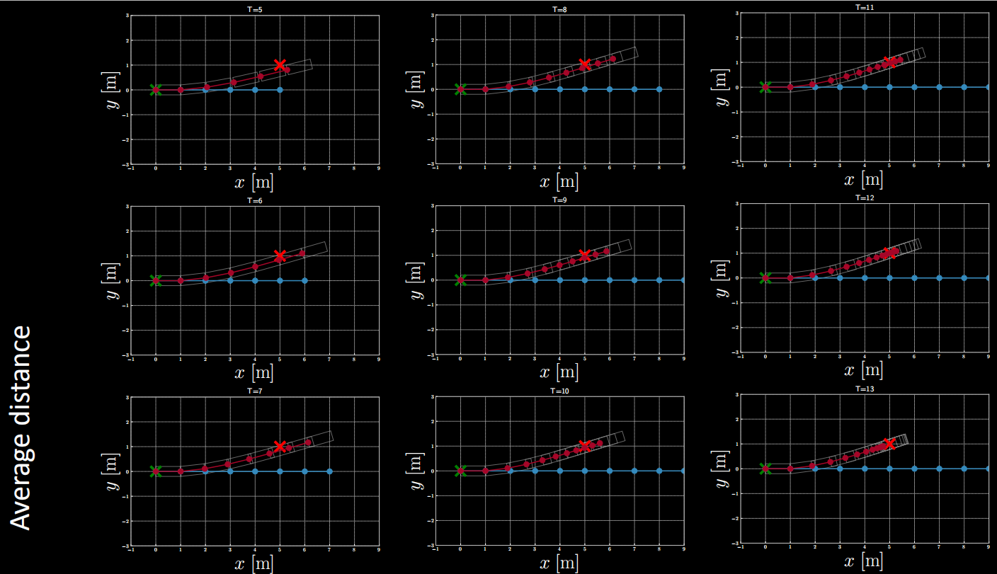
Figure 15: Cost Example: Average Distance

$(2)$ Cost Example: Softmin

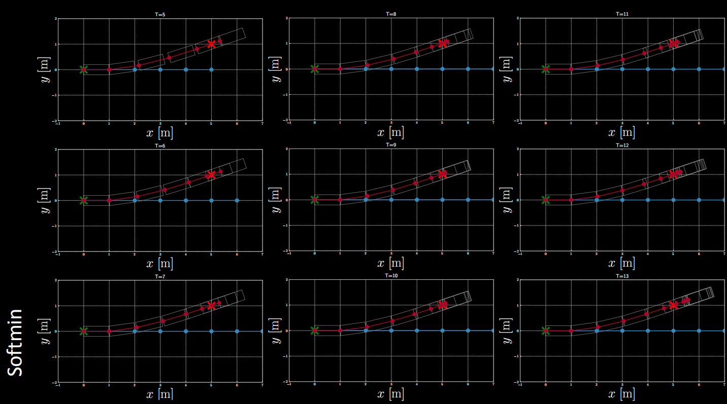
Figure 16: Cost Example: Softmin

Different forms of cost functions can be explored through experimentation.

Optimization_Path_Planner-Notebook

In this notebook, we use tri-cycle as an example as well.

Define kinematic model of a tricycle $\dot{\vx}=f(\vx,\vu)$.

• $\vx$ represents state: ($x$, $y$, $θ$, $s$)
• $\vu$ represents control: ($ϕ$, $a$)
• We feed $\vx[t-1]$ and $\vu[t]$ to obtain the next state $\vx[t]$

def f(x, u, t=None):
    L = 1  # m
    x, y, θ, s = x

    ϕ, a = u
    f = torch.zeros(4)
    f[0] = s * torch.cos(θ)
    f[1] = s * torch.sin(θ)
    f[2] = s / L * torch.tan(ϕ)
    f[3] = a
    return f

Define several cost functions

As mentioned above, cost functions can take various forms. In this notebook, we list 5 kinds as follows:

• vanilla_cost: Focuses on the final position
• cost_with_target_s: Focuses on the final position and final zero speed.
• cost_sum_distances: Focuses on the position of every step, and minimizes the mean of the distances.
• cost_sum_square_distances: Focuses on the position of every step, and minimizes the mean of squared distances.
• cost_logsumexp: The distance of the closest position should be minimized.

def vanilla_cost(state, target):
    x_x, x_y = target
    return (state[-1][0] - x_x).pow(2) + (state[-1][1] - x_y).pow(2)

def cost_with_target_s(state, target):
    x_x, x_y = target
    return (state[-1][0] - x_x).pow(2) + (state[-1][1] - x_y).pow(2)
                                       + (state[-1][-1]).pow(2)

def cost_sum_distances(state, target):
    x_x, x_y = target
    dists = ((state[:, 0] - x_x).pow(2) + (state[:, 1] - x_y).pow(2)).pow(0.5)
    return dists.mean()

def cost_sum_square_distances(state, target):
    x_x, x_y = target
    dists = ((state[:, 0] - x_x).pow(2) + (state[:, 1] - x_y).pow(2))
    return dists.mean()

def cost_logsumexp(state, target):
    x_x, x_y = target
    dists = ((state[:, 0] - x_x).pow(2) + (state[:, 1] - x_y).pow(2))#.pow(0.5)
    return -1 * torch.logsumexp(-1 * dists, dim=0)

Define path planning with cost

• The optimizer is set to be SGD.
• Time interval T is set to be 1s.
• We need to compute every state from the initial state by the following code:

  x = [torch.tensor((0, 0, 0, s),dtype=torch.float32)]
  for t in range(1, T+1):
      x.append(x[-1] + f(x[-1], u[t-1]) * dt)
  x_t = torch.stack(x)
  

• Then compute the cost:

  cost = cost_f(x_t, (x_x, x_y))
  costs.append(cost.item())
  

• Implement backprop and update $\vu$

  optimizer.zero_grad()
  cost.backward()
  optimizer.step()
  

• Now we can feed values to path_planning_with_cost to obtain inference results and plot trajectories. Example:

  path_planning_with_cost(
      x_x=5, x_y=1, s=1, T=5, epochs=5,
      stepsize=0.01, cost_f=vanilla_cost, debug=False
  )