Joint Embedding Methods - Contrastive

Visual Representation Learning

Representation learning trains a system to produce the representations required for feature detection or classification from raw data. Visual representation learning is about the representations of images or videos in particular.

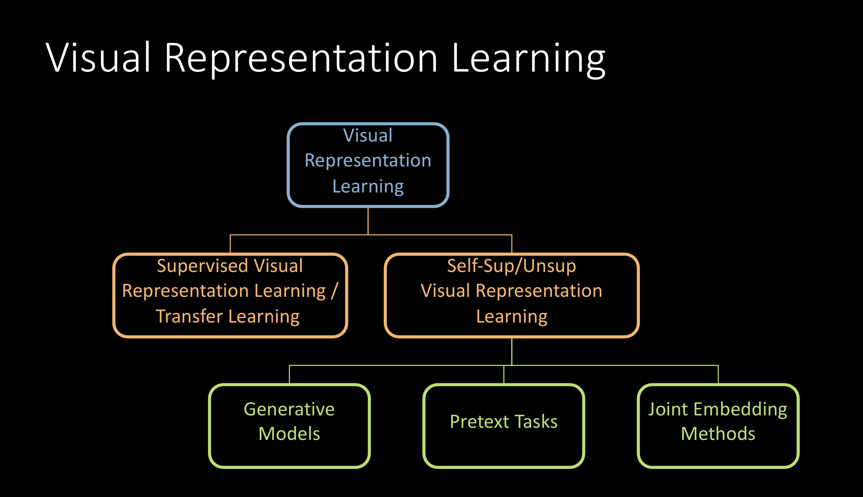
Fig. 1: Visual Representation Learning

This can be broadly classified as shown above and the focus of the lecture would be on self-supervised visual representation learning.

Self-supervised Visual Representation Learning

It is a two stage process comprising pretraining and evaluation

Step1: Pretraining

Uses a large amount of unlabeled data to train a backbone network. Different methods will produce the backbone network differently

Step2: Evaluation

It can be performed in two ways: feature extraction and finetuning. Both these methods generate representation from ​​the image and then use it to train DsTH ( Downstream Task Head ). The learning of the downstream task would thus be in the representation space instead of the image space. The only difference between the two methods is the stop gradient before the encoder. In finetuning, we can change the encoder unlike in feature extraction.

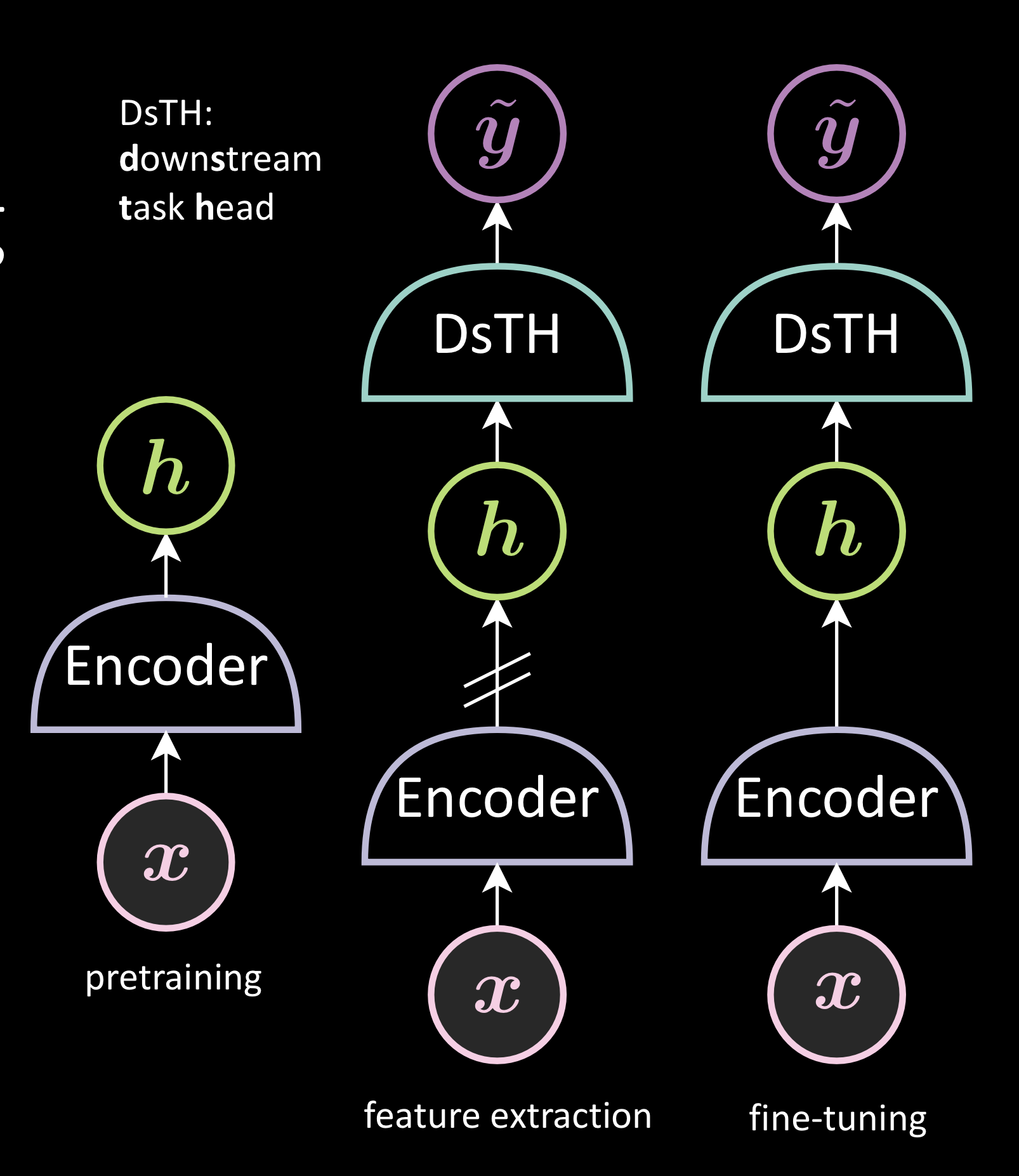
Fig. 2: Self-supervised Visual Representation Learning

Generative Models

The popular one is the denoising autoencoder. You train the model to reconstruct the original image from the noisy image. After the training, we retain the encoder for the downstream task.

Issues:

The model tries to solve a problem that is too hard. For example: For a lot of downstream tasks, you don’t have to reconstruct the image, which is a tougher problem than the downstream task itself. Also, sometimes the loss function is not good enough. For example: the Euclidean distance used as a reconstruction loss metric isn’t a good metric for comparing the similarity between two images.

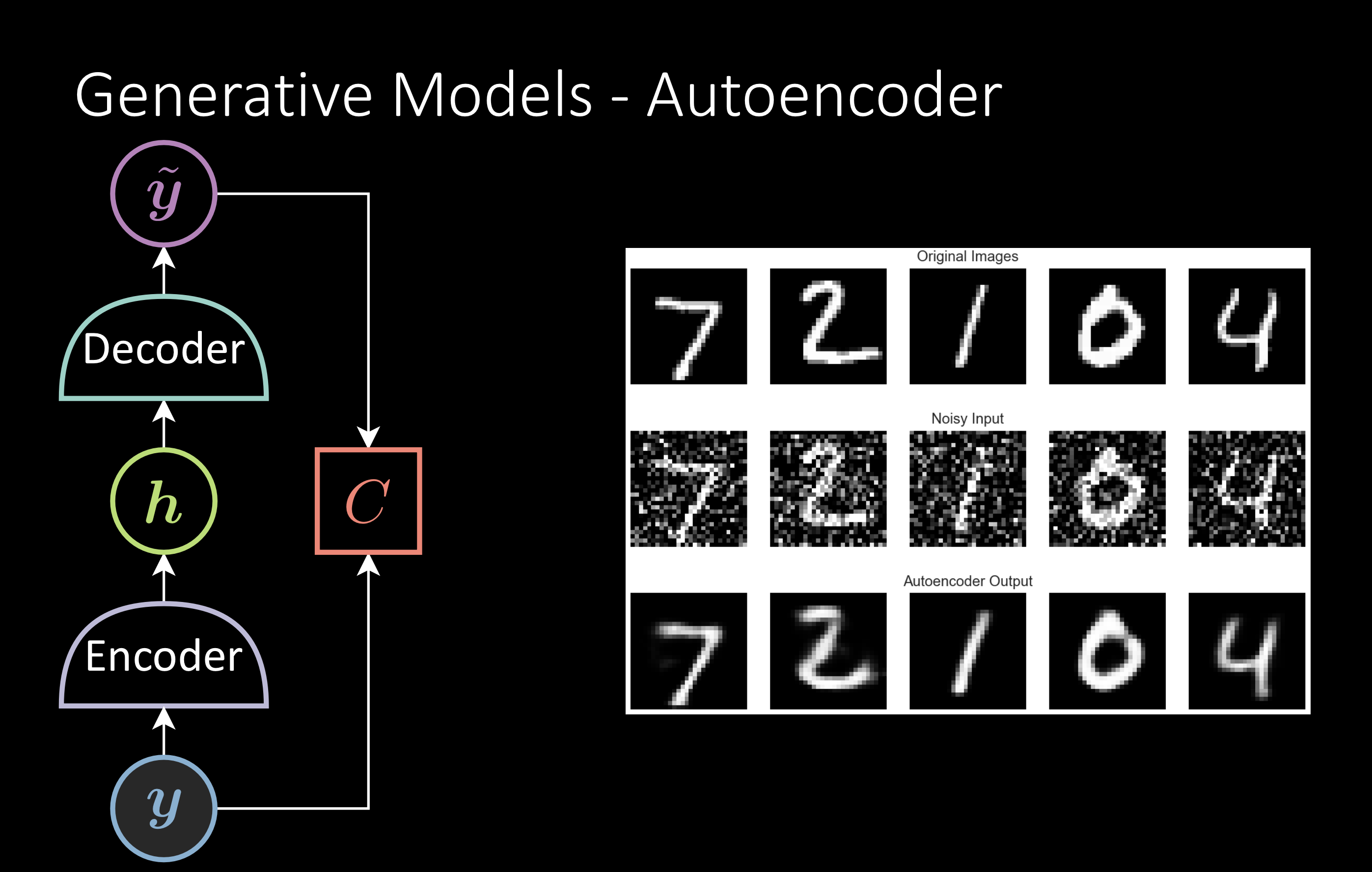
Fig. 3: Generative Models - Autoencoder

Pretext Tasks

It’s almost the same as above but you train the model to figure out a smart way to generate pseudo labels. For example: Given the image of a tiger, the shuffled image is the input x, and the output y would be the correct way of labeling the patches. The network successfully reinventing the patches indicates that it understands the image.

Issues:

Designing the pretext task is tricky. if you design the task too easy, the network won’t learn good representation. But if you design the task hard, it can become harder than the downstream task and the network wouldn’t be trained well. Also, the representations generated via this method will be tailored to the specific downstream task.

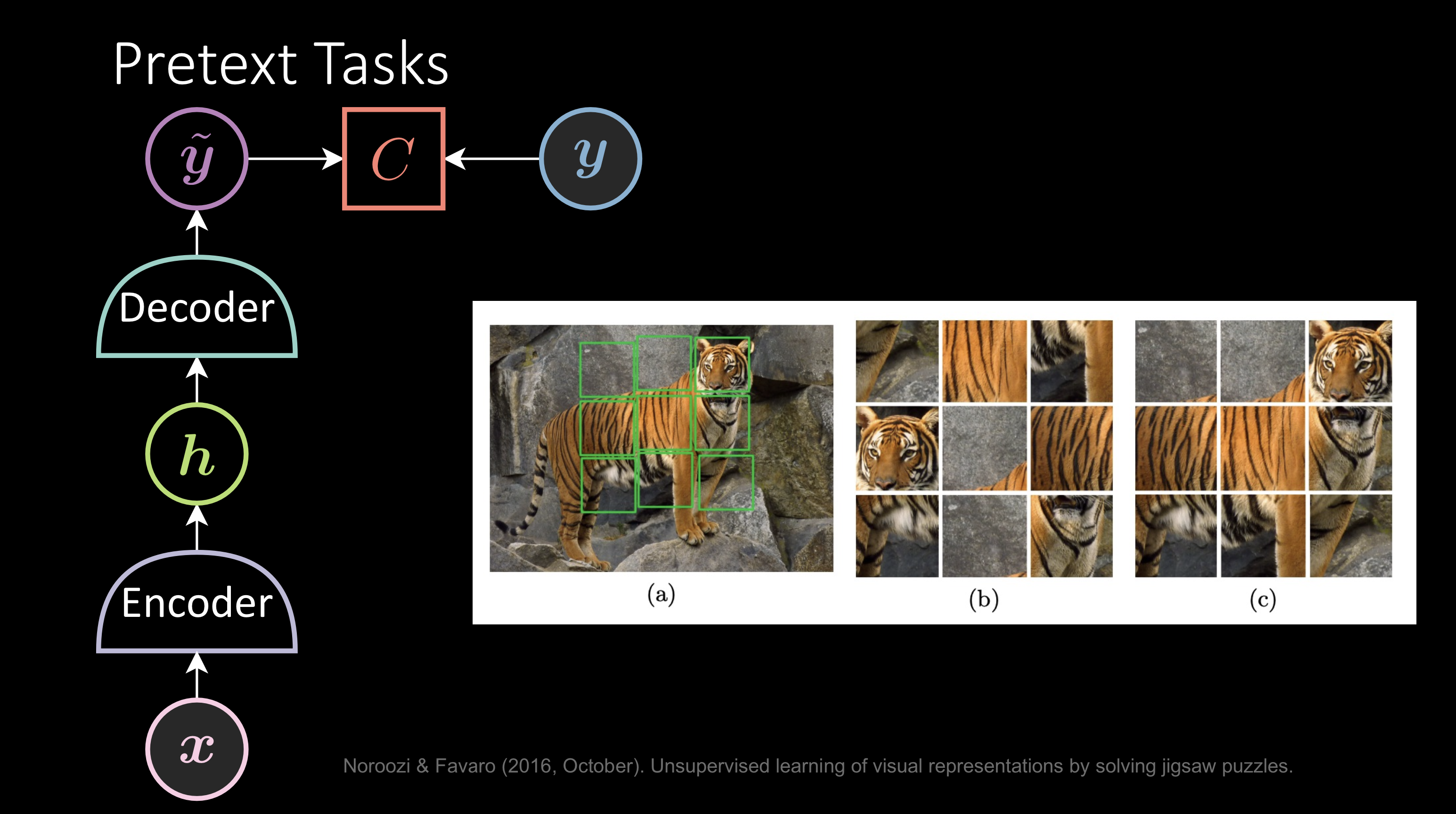
Fig. 4: Pretext Tasks

Joint Embedding Methods

Joint Embedding methods try to make their backbone network robust to certain distortions and are invariant to data augmentation.

As an example, as shown in the image below, for an image of a dog, you take two distorted versions of the image, then encode them with your backbone network to generate representations and you make them to be close to each other. Thus, ensuring the two images share some semantic information.

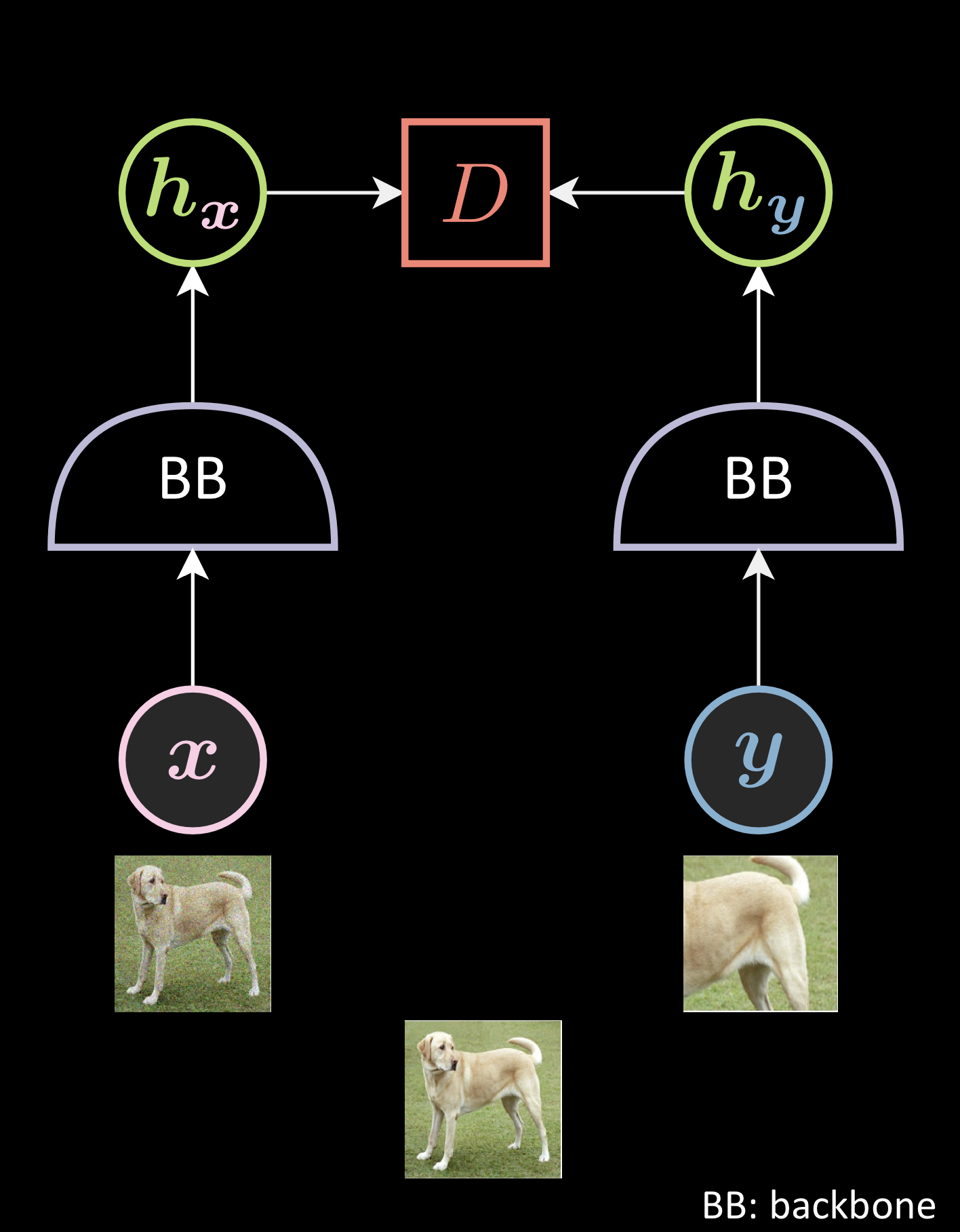
Fig. 1: Data Augmentation in JEM

They also prevent trivial solutions. The network could collapse with just the above condition, as the network can become invariant not only to distortions but to the input altogether i.e., irrespective of the input, it could generate the same output. JEMs try to prevent this trivial solution in different ways.

Instead of considering only local energy ( between two pairs of distorted images ), these methods get a batch of the images and ensure that the collection of the representation, $\green{H}_{\vx}$, doesn’t have the same rows or columns. ( which is the trivial solution )

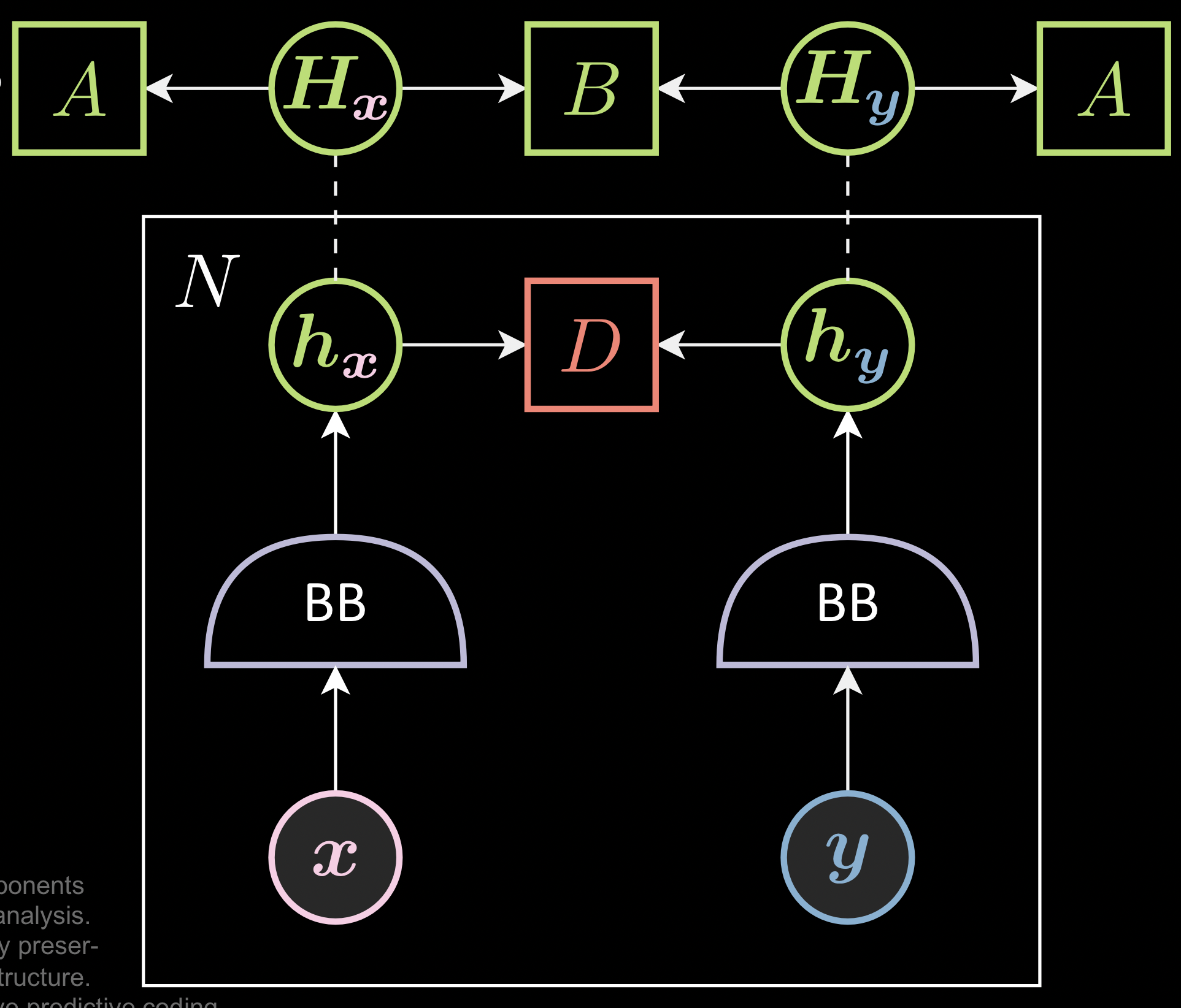
Fig. 2: Preventing Trivial Solutions in JEM

Components:

Every Joint Embedding Method has the following components:

1. Data augmentation ( $\vx$ and $\vy$ ): The way you generate the two distorted versions of the image.
2. Backbone Network ( $\lavender{BB}$ ) - The definition of the backbone
3. Energy function ( $\red{D}$ ) - The definition of the distance between the two representations.
4. Loss functionals ( $\green{A}$ and $\green{B}$ ) - The definition of the loss functionals calculated per batch of size N.

Joint Embedding Loss Functions:

Joint Embedding Loss Functions contain two components:

1. A term that pushes the positive pair closer
2. An (implicit) term that prevents the trivial solution (constant output) - implicit because a lot of “other methods” do not have an explicit term to prevent the trivial solution.

To make the training stable, people usually normalize the embeddings or put a hinge on the loss function to prevent the norm of embeddings from becoming too large or too small

Training Methods

The training methods can be further classified into the following four types:

1. Contrastive methods
2. Non-Contrastive methods
3. Clustering methods
4. Other methods

We now go into the details of each of these methods

Contrastive methods

Contrastive methods push positive pairs closer and negative pairs away. More details about the contrastive methods including MoCo, PIRL, and SimCLR have been discussed here.

The InfoNCE loss function:

Both SimCLR and MoCO use the InfoNCE loss function.

The first term indicates the similarity between positive pairs and the second term is the softmax between all the negative pairs. We would like to minimize this whole function.

Notice that it gives different weights to different negative samples. The negative pair that has high similarity is pushed much harder than the negative pair with low similarity because there’s a softmax. Also, the similarity measurement here is the inner product between the two representations, and to prevent the gradient explosion, the norm is normalized. Thus, even if the vector grew long, the term ensures that it is a unit vector.

Memory Bank:

As already mentioned, these models require negative samples. However, finding negative pairs becomes difficult as the embedding spaces become large.

To handle this, SimCLR and MoCO use large batch sizes to find the samples. The difference between SimCLR and MoCO is the way they deal with the large batch size. SimCLR uses 8192 as the batch size. However, MoCO tries to solve the requirement of a large batch size without actually using a large batch size by using a memory bank. It uses a small batch size but instead of using negative samples from only the current batch, it collects them even from previous batches. For example: with a 256 batch size, aggregating the previous 32 batches of negative samples results essentially in a batch size of 8192. This method saves memory and avoids the effort to generate the negative samples again and again.

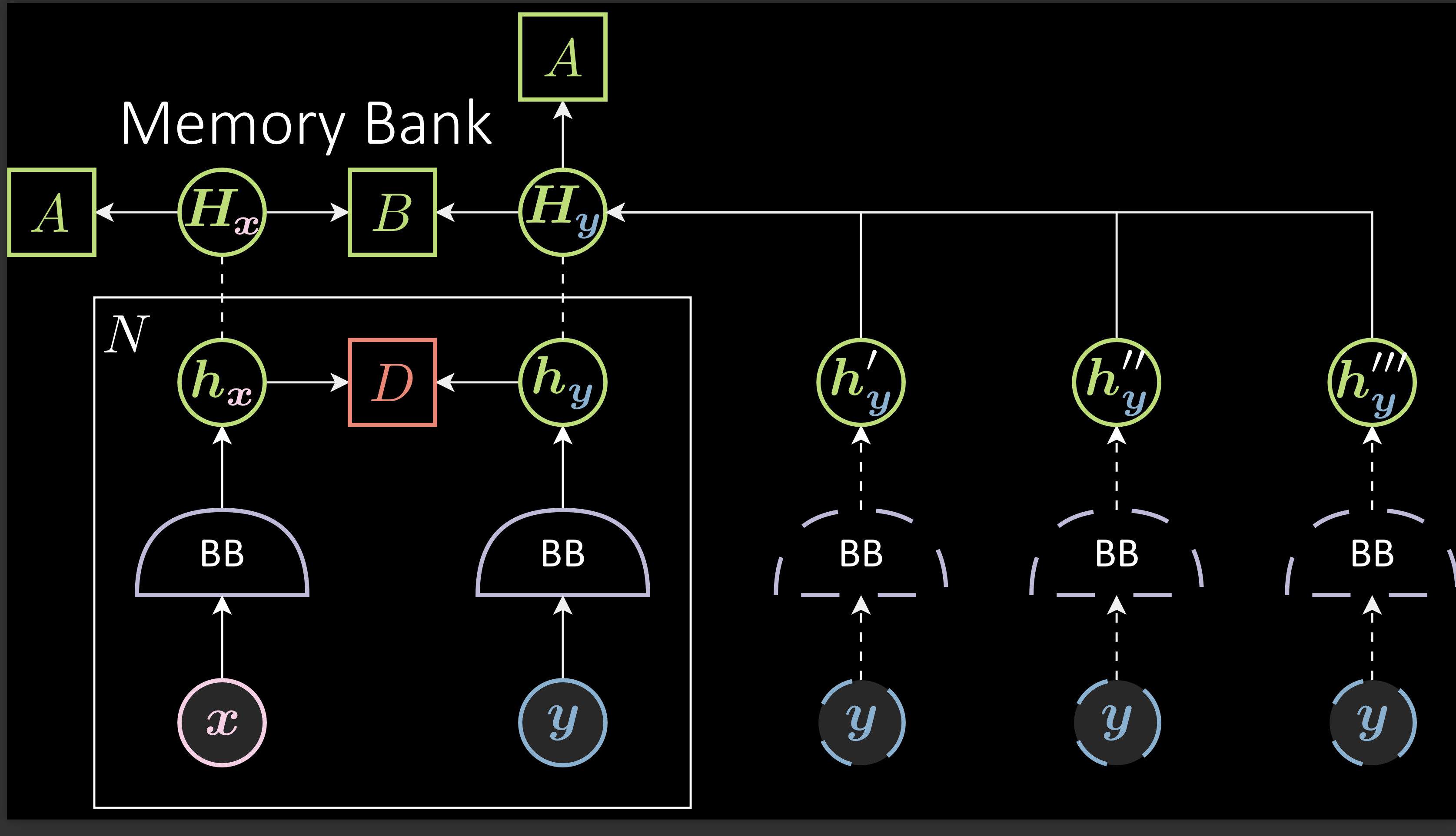
Fig. 4: Memory Bank

Issue: Because B is updated every step, the backbone is updated every step, and thus, after a while, the old negative samples are not valid anymore and can lead to a decrease in performance. To avoid this, MoCO uses a momentum backbone that slows down the training of the right backbone. In that case, the difference between the older momentum backbone and the new momentum backbone is not that different, retaining the validitiy of the negative sample even after a while.

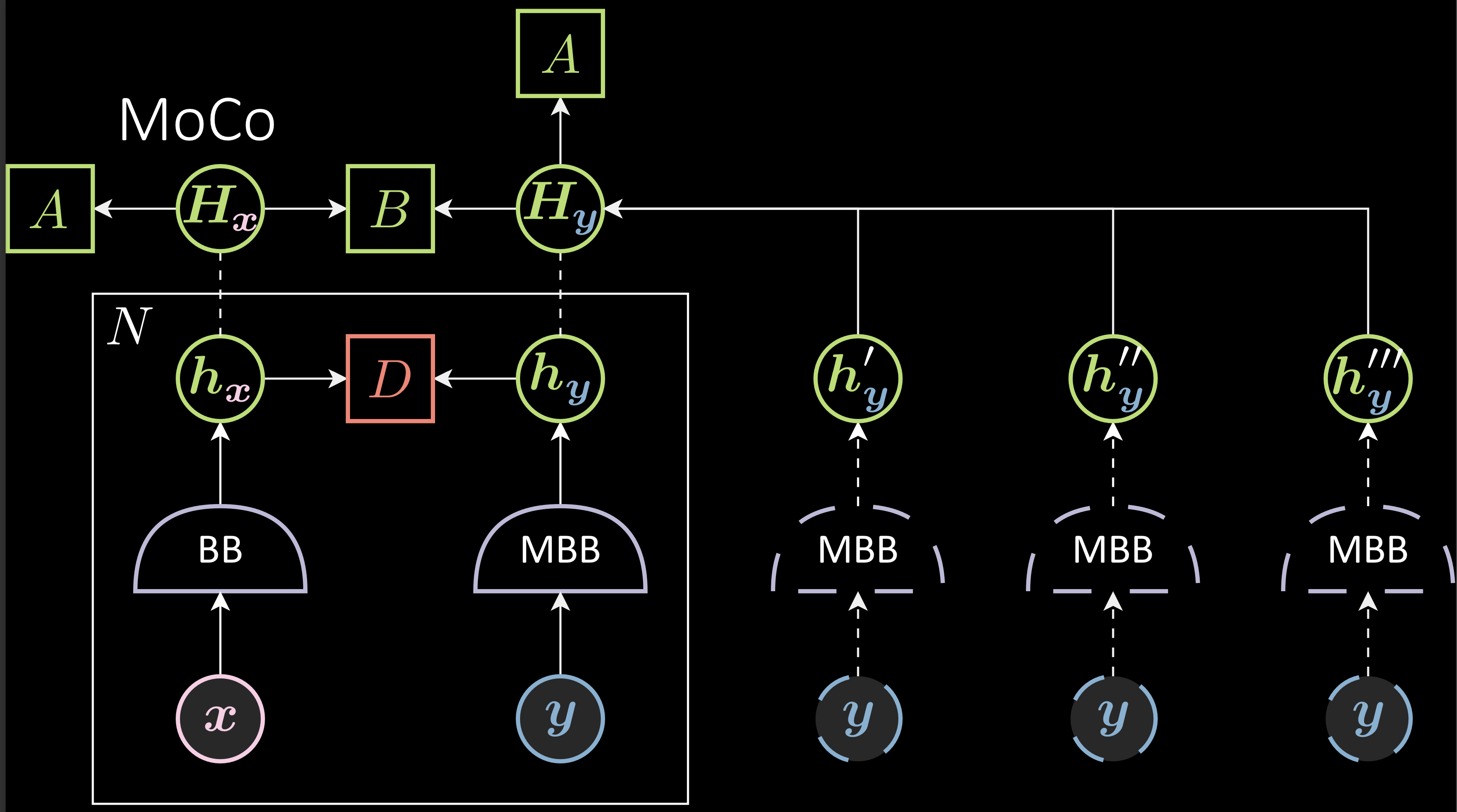
Fig. 5: Memory Bank with Momentum Backbone

$\vartheta_{t+1}$ ( momemtum backbone’s parameter ) is an exponential moving average of $\theta_{t}$. The learning rate of $\vartheta$ is $( 1 - m )* \eta$. High values of $m$ will make the $\vartheta_{t}$ stable. $m$ =1 will make $\vartheta_{t}$ basically untrained. If $m$ is very small like 0, $\vartheta_{t+1}$ is $\theta_{t+1}$.

Disadvantages of Contrastive methods:

In practice, people found out that contrastive methods need a lot of setup to make them work. They require techniques such as weight sharing between the branches, batch normalization, feature-wise normalization, output quantization, stop gradient, memory banks etc.,.This makes it hard to analyze. Also, they are not stable without the use of those techniques.