SEER, AVID + CMA, Distillation, Barlow Twins

SEER: Learning from uncharted Images

Compared to Imagenet dataset, real world images may have different distributions (cartoons, memes) and may or may not have a prominent object. In order to verify if the models work well on images outside of Imagenet dataset we decided to test Swav method on large scale data. SEER is Swav method tested on billions of unfiltered images.

Following graph compares the fine tune performance of the four models when transferred to Imagenet. Using SEER method, a model can be trained with more than a billion parameters which are going to transfer really well to Imagenet.

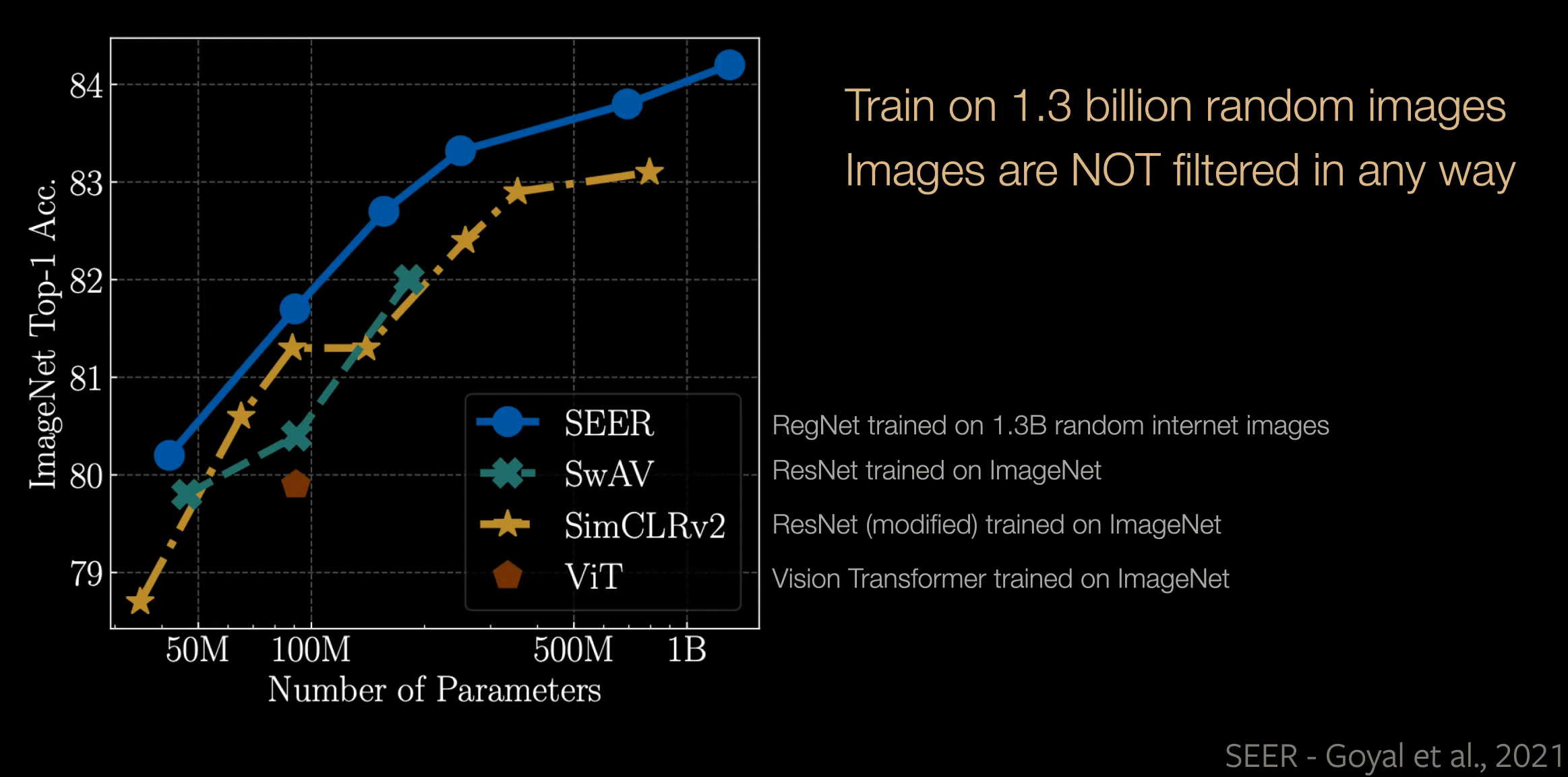
Figure 1 Comparing SEER to other methods on ImageNet data

As shown in the following table, the performance of SEER is comparable to the networks trained on curated data with weak supervision.

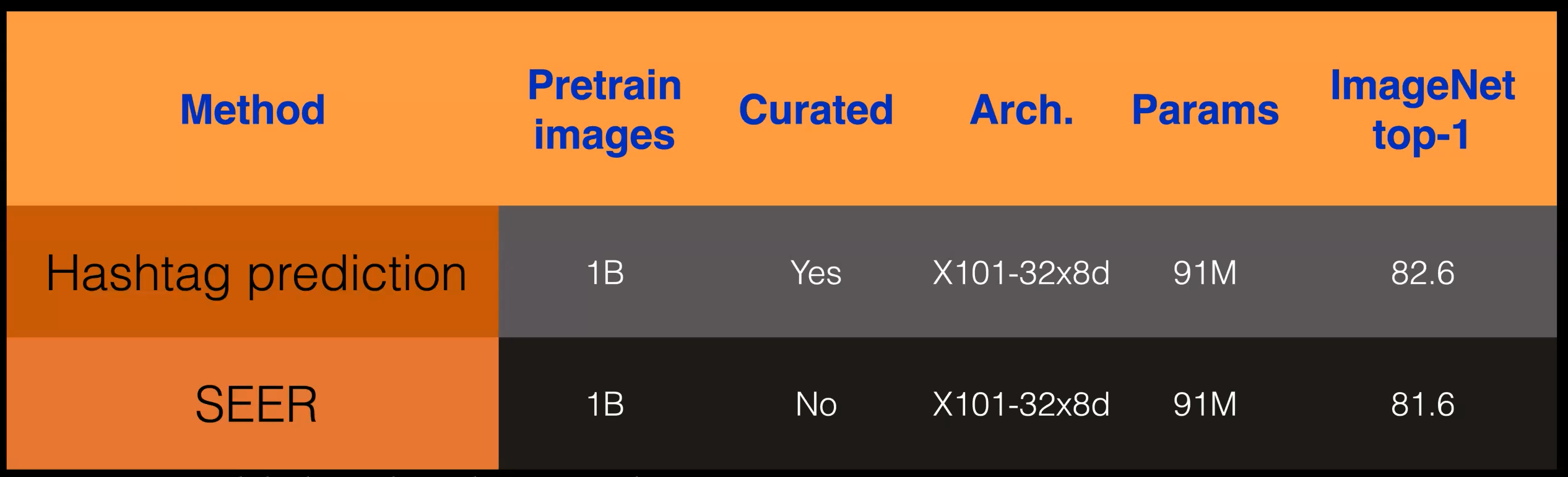
Figure 2 SEER performance vs weak supervision model

AVID + CMA

Audio Visual Instance Discrimination with Cross Modal Agreement is a method that combines contrastive learning and clustering techniques.

For contrastive leaning on an Audio-Video dataset, when the (audio-video) inputs are passed to the two encoders ($f_a, f_v$) we will get two embeddings (audio and video). The embeddings from the same sample should be close in feature space compared to embeddings from different samples.

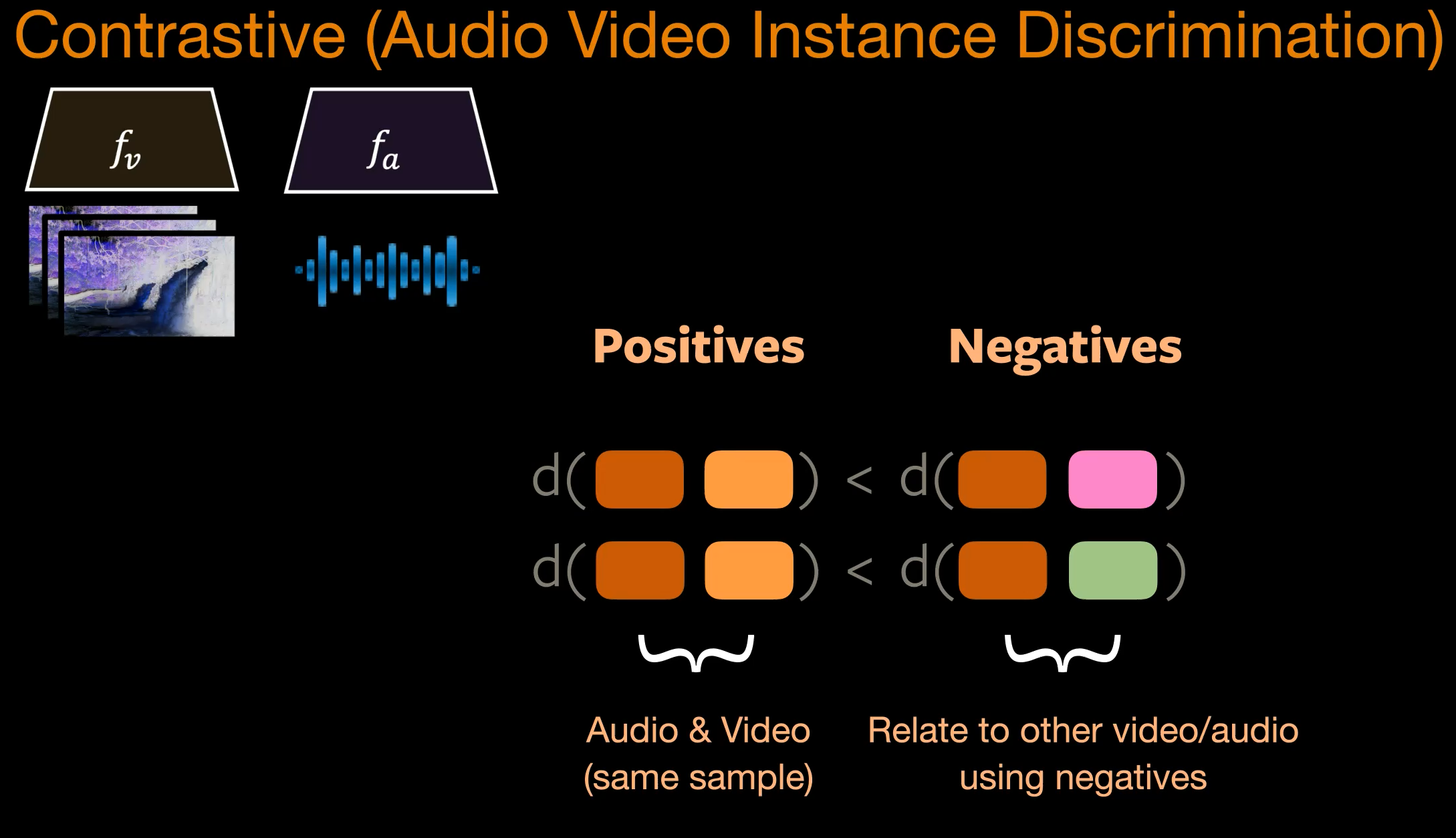
Figure 3 AVID: Audio Video Instance Discrimination

To introduce the clustering, the notion of the positives and negatives is expanded as shown in the following image. Computing the similarities in the video and audio embeddings from a reference point to all the other samples results in Positive Set and Negative Set. A sample falls into positive set when both its audio and video embeddings are similar to the reference embeddings.

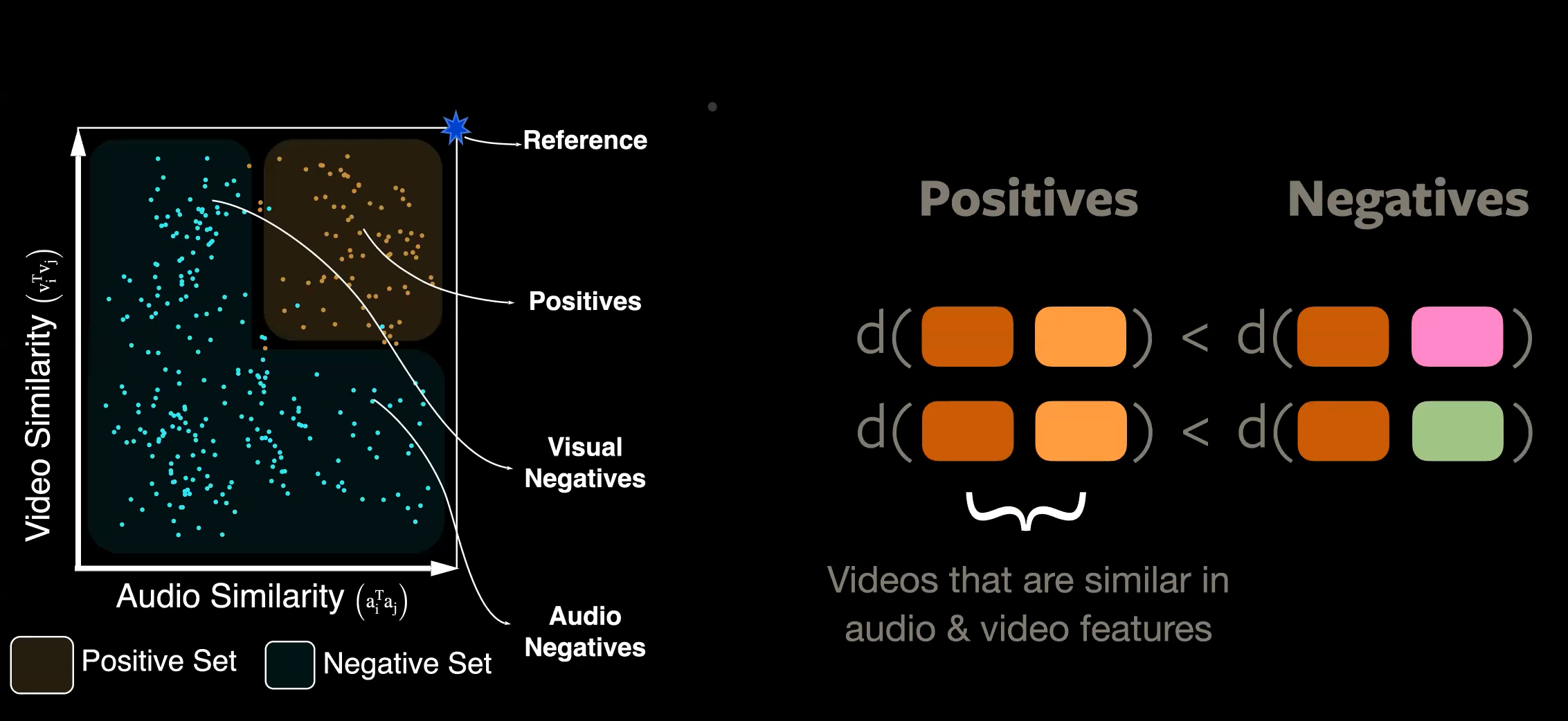
Figure 4 CMA: Cross-Modal Agreements

Distillation

Distillation methods are similarity maximization based methods. Like other SSL methods distillation tries to prevent trivial solutions. It does so by asymmetry in two different ways.

• Asymmetric learning rule between student teacher
• Asymmetric architecture between student teacher

BYOL

BYOL is a distillation technique whose architecture is shown below.

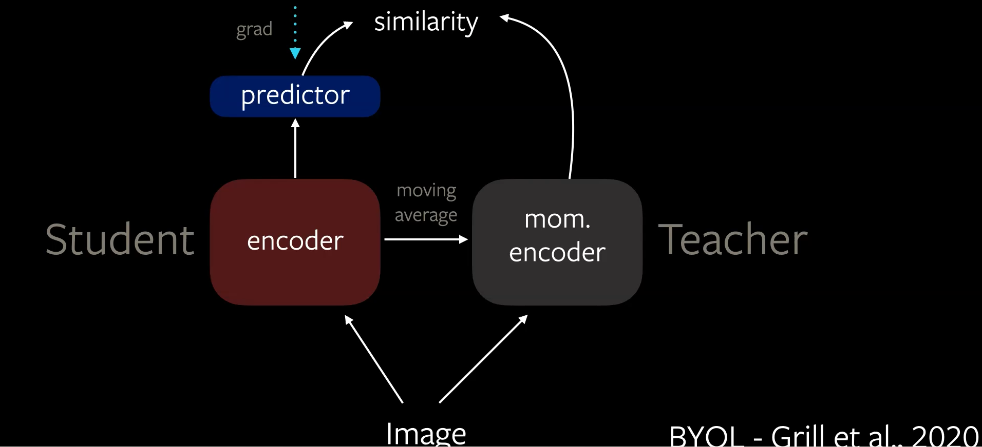
Figure 5 BYOL architecture

There is an asymmetry in architecture between student teacher as student has an additional prediction head. The gradient backpropagation only happens through Student encoder clearly creating an asymmetry in learning rate. In BYOL there is an additional source of asymmetry which is in weights of student encoder and teacher encoder. Teacher encoder is created as moving average of student encoder. These asymmetries will prevent the model from trivial solutions.

SimSiam

Recent studies showed that all the three sources of asymmetry discussed in BYOL are not needed to prevent the trivial solutions. In SimSiam architecture the student and teacher share the same set of weights and there are two sources of asymmetry.

• In architecture of student encoder with an additional predictor head.
• In learning rate, when backpropagating the gradients are passed only through student encoder but not the teacher encoder. After each epoch, the weights of student encoder are copied to the teacher encoder.

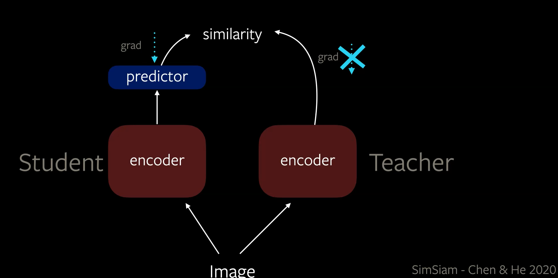
Figure 6 SimSiam architecture

Barlow Twins

Hypothesis from information theory

The efficient coding hypothesis was proposed by Horace Barlow in 1961 as a theoretical model of sensory coding in the brain. Within the brain, neurons communicate with each other by sending electrical impulses called spikes. Barlow hypothesised that the spikes in the sensory system form a neural code for efficiently representing sensory information. By efficient, Barlow meant that the code minimises the number of spikes needed to transmit a given signal.

Implementation

A successful approach to Self-Supervised-Learning (SSL) is to learn representations which are invariant to distortions of the input sample. However, a recurring problem with this approach is the existence of trivial constant solutions.

The Barlow Twins method proposes an objective function that naturally avoids such collapse by measuring the cross-correlation matrix between the outputs of two identical networks fed with distorted versions of a sample and making them as close as possible to the identity matrix.

Barlow’s redundancy-reduction principle applied to a pair of identical networks. The objective function measures the cross-correlation matrix between the output features of two identical networks fed with distorted versions of a batch of samples and attempts to bring this matrix close to the identity. This causes the representation vectors of distorted versions of a sample to be similar, while minimizing the redundancy between the components of these vectors (Figure 7).

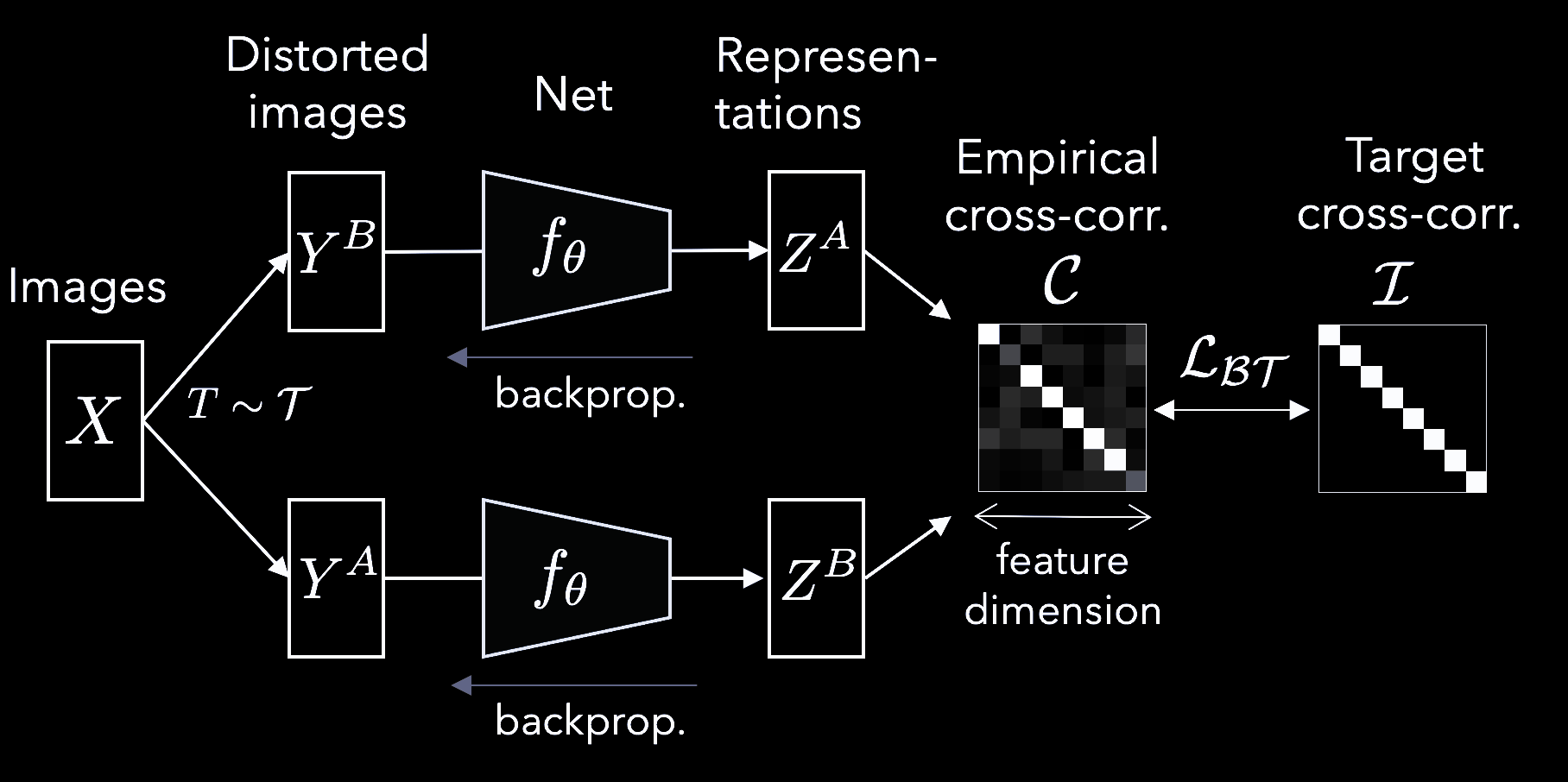
Figure 7 Barlow-Twins Architecture

More formally, it produces two distorted views for all images of a batch $X$. The distorted views are obtained via a distribution of data augmentations $\mathcal{T}$. The two batches of distorted views $Y^A$ and $Y^B$ are then fed to a function $f_{\vtheta}$, typically a deep network with trainable parameters $\vtheta$, producing batches of representations $Z^{A}$ and $Z^{B}$ respectively.

The loss function $\mathcal{L_{BT}}$ contains a invariance and redundancy reduction:

where $\lambda$ is a constant controlling the importance of the first and second terms of the loss, and where $\mathcal{C}$ is the cross-correlation matrix computed between the outputs of the two identical networks along the batch dimension:

where $b$ indexes batch samples and $i,j$ index the vector dimension of the networks’ outputs. $\mathcal{C}$ is a square matrix with size the dimensionality of the network’s output. In other words

Intuitively, the invariance term of the objective, by trying to equate the diagonal elements of the cross-correlation matrix to 1, makes the representation invariant to the distortions applied. The redundancy reduction term, by trying to equate the off-diagonal elements of the cross-correlation matrix to 0, decorrelates the different vector components of the representation. This decorrelation reduces the redundancy between output units, so that the output units contain non-redundant information about the sample.