Generative Models - Autoencoders
🎙️ Alfredo CanzianiRecap: Predictive Latent Variable Model
As we know latent variables are useful in providing additional information that help in predicting multiple values of the target $\vy$, associated with the input $\cx$. We have seen earlier, in order to predict the target variable $\vy$ from latent variable $\cz$, the energy function is given as,
\[\red{E}(\vy,\cz) = [y_1 - g_1(\cz)]^2 + [y_2 - g_2(\cz)]^2, \vy \in \boldsymbol{Y}\]To be clear, we show the unit of $\boldsymbol{g}$:
\[\boldsymbol{g} = [g_{1}, g_{2}]^\top, \mathbb{R} \rightarrow \mathbb{R}^{2} \\ \boldsymbol{g}(\cz) = [w_{1}\cos(\cz), w_{2}\sin(\cz)]\]In this case, the latent variable $\cz$ is one dimensional. However, if the $\vz$ has a higher dimension, this could lead to an energy function of $0$ everywhere. Hence, in order to ensure lower energy values for more compatible predictions we introduce a regularized factor.
Training recap
Given an observation $\vy$, training the regularised latent variable model
\[\red{E}(\vy,\vz) = \red{C}(\vy,\vytilde) + \red{R}(\vz)\]where $\vytilde = \Dec(\vz)$,
- compute
- Minimise
At zero temperature limit,
- Compute
- Minimise
Target propagation
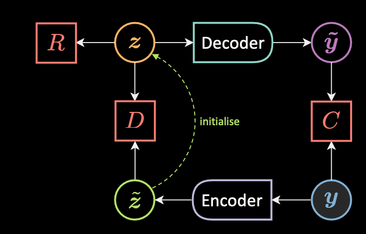
Fig. 1: Target propagation
Fig. 1 shows the architecture of target propagation. Given an observation $\vy$, we first compute $\vztilde$ which is the initial guess of the latent variable $\vz$
\[\vztilde = \Enc(\vy)\]We then initialize $\vz$ to $\vztilde$, here we must ensure that these values are not too far apart from each other.
\[\vzcheck = \underset{\vz}{\arg\min}{\red{E}(\vy,\vz)} \\ \red{E}(\vy,\vz) = \red{C}(\vy, \vytilde) + \red{R}(\vz) + \red{D}(\vz,\vztilde)\]We now minimise the loss functional in two steps, minimise $\mathcal{L}(\red{F}_{\infty}(\cdot), \vect{\blue{Y}})$:
\[\vtheta_{\Dec} = \vtheta_{\Dec} - \triangledown_{\vtheta_{\Dec}}\red{C}(\vy,\vytilde)\\ \\ \vtheta_{\Enc} = \vtheta_{\Enc} - \triangledown_{\vtheta_{\Enc}}\red{D}(\vzcheck,\vztilde)\]In this way $\vz$ is constrained in taking only a set of values.
Autoencoder (AE)
An autoencoder is a type of artificial neural network used to learn efficient data encodings in an unsupervised manner. The aim is to first learn encoded representations of our data and then generate the input data (as closely as possible) from the learned encoded representations. Thus, the output of an autoencoder is its prediction for the input.
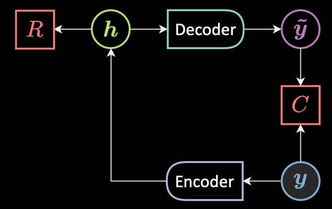
Fig. 2: Architecture of a basic autoencoder
Fig. 2 shows the architecture of a basic unconditional autoencoder. To summarize at a high level, a very simple form of AE is as follows:
- First, the autoencoder takes in an input and maps it to a hidden state through an affine transformation $\vh = f(\mW{_h} \vy + \vb{_h})$, where $f$ is an (element-wise) activation function. This is the encoder stage. Note that $\vh$ is also called the code.
- Next, $\vytilde = g(\mW{_y} \vy + \vb {_y})$, where $g$ is an activation function. This is the decoder stage.
- Finally, the energy is the sum of the reconstruction and the regularization, $\red{F}(\vy) = \red{C}(\vy,\vytilde)+ \red{R}(\vh)$.
Reconstruction costs
When the input is real-valued we use mean squared error loss,
\[\red{C}(\vy,\vytilde) = \Vert \vy - \vytilde \Vert^{2} = \Vert{\vy - \Dec[\Enc(\vy)]}\Vert^{2}\]When the input is categorical we use cross entropy loss,
\[\red{C}(\vy,\vytilde) = -\sum_{i = 1}^{n} \vy_i \log(\vytilde_i) + (1 - \vy_i)\log(1 - \vytilde_i)\]Loss functional
The loss functional is the average of the per sample loss.
\[\mathcal{L}(\red{F}(\cdot), \vect{\blue{Y}}) = \frac{1}{m} \sum_{j = 1}^{m} \ell(\red{F}(\cdot),y^{(j)}) \in \mathbb{R} \\ \ell_\text{energy}(\red{F}(\cdot),\vy) = \red{F}(\vy)\]Under-/over-complete hidden layer
When the dimensionality of the hidden layer is less than the dimensionality of the input then it is under complete hidden layer. When the dimensionality of the hidden layer is greater than the dimensionality of the input then it is over complete.
The dimensionality of the hidden layer is larger than the input so that they can be linearly separable. However, this can lead to a collapsed representation. Since by reconstructing the input, the model can copy all the features. In order to avoid this there are a few techniques such as denoising autoencoder, contractive autoencoder, variation autoencoder, etc.
Denoising Autoencoder
Denoising Autoencoder is a contrastive technique. Fig. 3 below shows the architecture and manifold of the denoising autoencoder and the intuition of how it works.
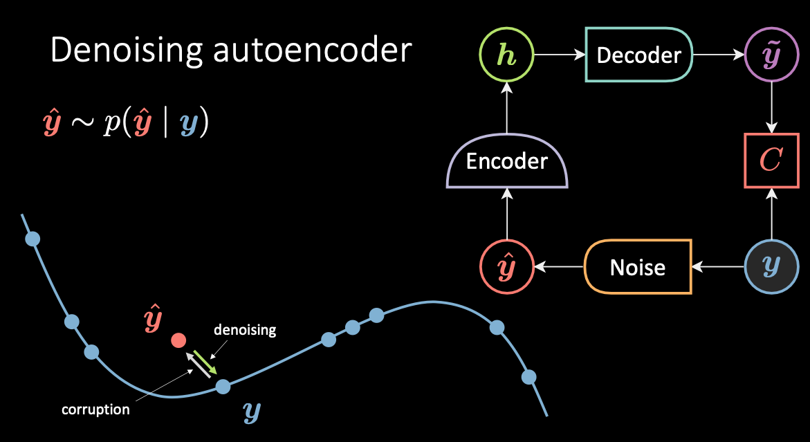
Fig. 3: Denoising Autoencoder
In this model, we corrupt the input data $\vy$, in blue, because it’s cold / low energy, and get the sample $\vyhat$, in red, because it’s hot / high energy. The energy associated to $\vytilde$ is squared euclidean distance from its original value. Then $\vytilde$ is encoded back to the hidden variable $\vh$ and then passed back to the decoder producing $\vytilde$ which should be close to the target $\vy$. Hence irrespective of what noise is added to the original data, the autoencoder needs to learn to separate the noise and retrieve the original value of $\vy$.
Contractive Autoencoder
A contractive autoencoder is an unsupervised deep learning technique that helps a neural network encode unlabelled training data. It makes this encoding less sensitive to small variations in its training dataset. This is accomplished by adding a regulariser, or penalty term, to whatever cost or objective function the algorithm is trying to minimize. The end result is to reduce the learned representation’s sensitivity towards the training input.
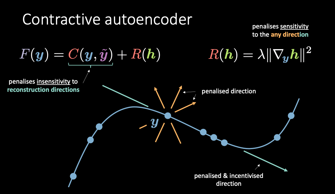
Fig. 4: Contractive autoencoder
As shown in Fig. 4, $\red{C}(\vy, \vytilde)$ penalises sensitivities to reconstructions along the manifold while $\red{R}(\vh)$ penalises how much the wiggling of $\vh$ comes from the wiggling of $\vy$. In this manner, you basically get to push up the energies only in the direction that are not used for the reconstruction.
Variational Autoencoder (VAE)
Intuition behind VAE and a comparison with classic autoencoders
Next, we introduce Variational Autoencoders (or VAE), a type of generative model. But why do we even care about generative models? To answer the question, discriminative models learn to make predictions given some observations, but generative models aim to simulate the data generation process. One effect is that generative models can better understand the underlying causal relations which leads to better generalization.
What’s the difference between variational autoencoder (VAE) and basic autoencoder (AE)?
Note that although VAE has “Autoencoders” (AE) in its name (because of structural or architectural similarity to auto-encoders), the formulations between VAEs and AEs are very different. Fig. 5 below shows the architectures of VAE and basic AE.
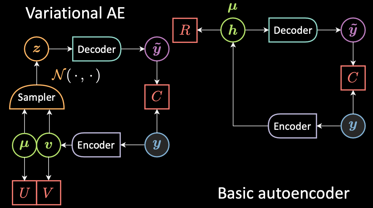
Fig. 5: VAE vs. Basic AE
For VAE:
- First, the encoder stage: we pass the input $\vy$ to the encoder. Instead of generating a hidden representation $\vh$ in AE, the hidden representation in VAE comprises two parts: $\vmu$ and $\vv$. And similar to using regularisation factor $\red{R}$ for $\vh$, we now use regularisation factors $\red{U}$ and $\red{V}$ for $\vmu$ and $\vv$, respectively.
- Next, we use a sampler to sample $\vz$ which is the latent random variable following a Gaussian distribution with $\vmu$ and $\vv$. Note that people use Gaussian distributions as the encoded distribution in practice, but other distributions can be used as well.
- Finally, $\vz$ is passed into the decoder to generate $\vytilde$.
- The decoder will be a function from $\orange{\mathcal{Z}}$ to $\mathbb{R}^{n}$: $\vz \mapsto \vytilde$.
In fact, for basic autoencoder, we can think of $\vh$ as just the vector $\vmu$ in the VAE formulation, with the variance set to zero. In short, the main difference between VAEs and AEs is that VAEs have a good latent space that enables generative process.
What’s the difference between variational autoencoder (VAE) and denoising autoencoder (DAE)?
Now let’s have compare the difference between VAE and DAE. See Fig. 6 below.
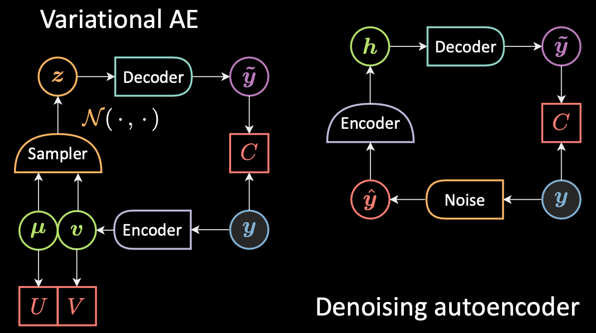
Fig. 6: VAE vs. Denoising AE
For DAE as we mentioned before, the sampling was happening between $\vy$, in blue, because it’s cold / low energy, and $\vyhat$, in red, because it’s hot / high energy. So we move the input and then we decode everything into $\vytilde$. For VAE we encode the input and we add noise in the hidden , so we just switch the position of the encoder in the sampler more or less.
The VAE objective (loss) function
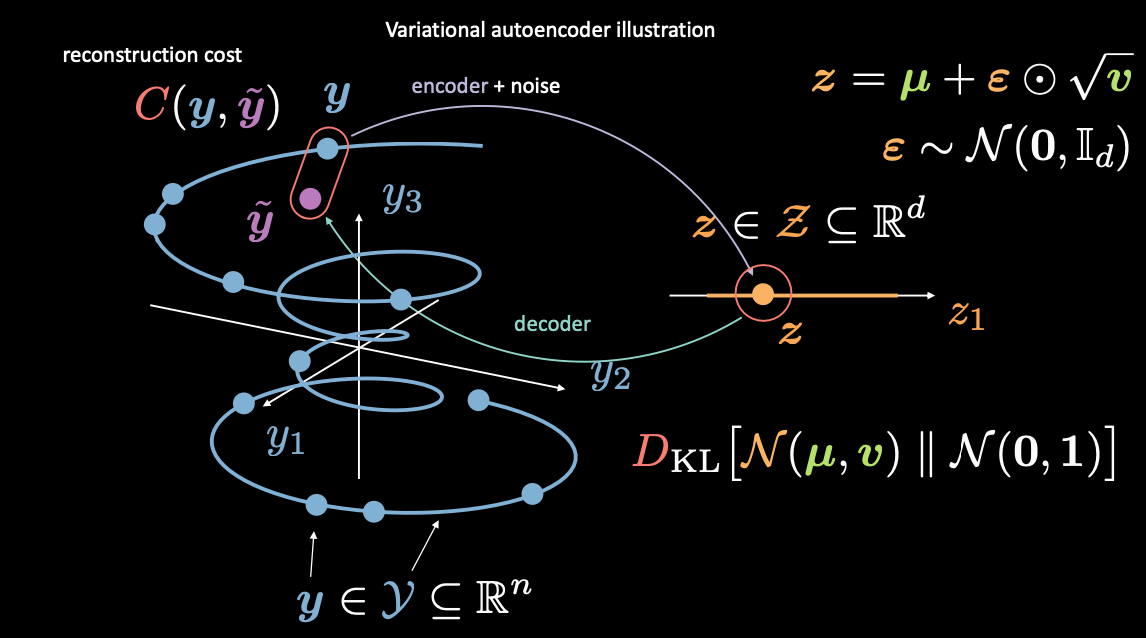
Fig. 7: Mapping from input space to latent space
First, we encode from input space (left) to latent space (right), through encoder and noise. Next, we decode from latent space (right) to output space (left). To go from the latent to input space (the generative process) we will need to either learn the distribution (of the latent code) or enforce some structure. In our case, VAE enforces some structure to the latent space.
As usual, to train VAE, we minimize a loss function. The loss function is therefore composed of a reconstruction term as well as a regularization term.
- The reconstruction term is on the final layer (left side of the figure). This corresponds to $\red{C}(\vy, \vytilde)$ in the figure.
- The regularization term is on the latent layer, to enforce some specific Gaussian structure on the latent space (right side of the figure). We do so by using a penalty term $\red{D}_{KL}(\orange{\mathcal{N}}(\vmu, \vv) \mathrel{\Vert} \orange{\mathcal{N}}(\boldsymbol{0}, \boldsymbol{1}))$. Without this term, VAE will act like a basic autoencoder, which may lead to overfitting, and we won’t have the generative properties that we desire.
Discussion on sampling $\vz$ (reparameterisation trick)
How do we add this noise as mentioned above? We here introduce reparameterisation trick. From above we know that, we sample from the Gaussian distribution, in order to obtain latent variable $\vz$. However, this is problematic, because when we do gradient descent to train the VAE model, we don’t know how to do backpropagation through the sampling module.
We can simply say that the new latent $\vz$ is going to be $\vmu$ which is the guess for the mean plus a epsilon that was sampled from a Gaussian whose amplitude is changed by the square root of the standard deviation $\vv$. So in this way, we can get gradients back flowing in these encoder.
Visualizing Latent Variable Estimates and Reconstruction Loss
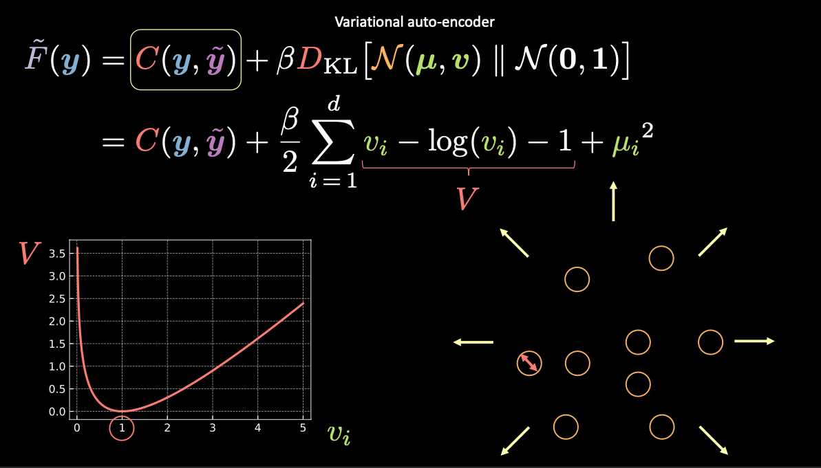
Fig. 8: Visualizing vector $z$ as bubbles in the latent space
In Fig. 8 above, each bubble represents an estimated region of $\vz$, and the arrows represent how the reconstruction term pushes each estimated value away from the others, which is explained more below.
As stated above, the Free Energy for the VAE contains two terms: a reconstruction term and a regularization term. We can write this as
\[\red{\tilde{F}}(\vy) = \red{C}(\vy, \vytilde) + \beta \red{D}_{\text{KL}}(\orange{\mathcal{N}}(\vmu, \vv) \mathrel{\Vert} \orange{\mathcal{N}}(\boldsymbol{0}, \boldsymbol{1}))\]To visualize the purpose of each term in the free energy, we can think of each estimated $\vz$ value as a circle in $2d$ space, where the centre of the circle is $\vmu$ and the surrounding area are the possible values of $\vz$ determined by $\vv$.
If there is an overlap between any two estimates of $\vz$, (visually, if two bubbles overlap) this creates ambiguity for reconstruction because the points in the overlap can be mapped to both original inputs. The first term $\red{C}(\vy, \vytilde)$ forces to reconstructing these bubbles to the correct locations.
- The reconstruction loss $\red{C}(\vy, \vytilde)$ will push the points away from one another such there is no overlap.
- Another option for $\red{C}(\vy, \vytilde)$ to avoid overlap is to make the variance zero and then there are just points other than bubbles so there’s no more overlap.
However, if we use just the reconstruction loss, the estimates will continue to be pushed away from each other and the system could blow up. This is where the penalty term comes in.
The penalty term
The second term is the relative entropy (a measure of the distance between two distributions) between a Gaussian, with mean $\vmu$ and variance $\vv$, and the standard normal distribution. If we expand this second term in the VAE loss function we get:
\[\red{D}_{\text{KL}}(\orange{\mathcal{N}}(\vmu, \vv) \mathrel{\Vert} \orange{\mathcal{N}}(\boldsymbol{0}, \boldsymbol{1})) = \frac{1}{2} \sum\limits_{i=1}^d \green{v_i} - \log{(\green{v_i})} - 1 + \green{\mu_i}^2\]where the expression in the summation has four terms. Let’s use $\red{V}$ for the first three terms.
\[\red{V} = \green{v_i} - \log{(\green{v_i})} - 1\]From the left bottom plot in Fig. 8 above, we can see that this expression is minimized when $\green{v_i}$ is 1. Therefore our penalty loss will keep the variance of our estimated latent variables at around 1. Visually, this means our “bubbles” from above will have a radius of around 1.
The last term, $\green{\mu_i}^2$, minimizes the distance between the bubbles and therefore prevents the “exploding” encouraged by the reconstruction term.
Note: The $\beta$ in the VAE loss function is a hyperparameter that dictates how to weight the reconstruction and penalty terms.
📝 Nandhitha Raghuram, Xinyi Zhao
25 March 2021