Speech Recognition and Graph Transformer Network I

Modern Speech Recognition

This section is a high level introduction to speech recognition and modern speech recognition specifically why it’s become so good, but what are some of the problems still.

• Automatic speech recognition has greatly improved since 2012
  • Machine performance can be as good or better than human level performance
• Speech recognition still struggles in
  • conversational speech
  • multiple speakers
  • lots of background noise
  • the accent of the speakers
  • certain features not well represented in the training data
• Pre 2012 speech recognition systems consisted of lots of many hand engineered components
  • larger dataset is not useful so datasets remain small
  • combining modules only at inference time instead of learning them together allowed for errors to cascade
  • researchers hard to know how to improve complex systems
• Post 2012 speech recognition systems improvements
  • replaced a lot of the traditional components
  • add more data
  • above two together work in a virtuous cycle

The CTC Loss

Given some input speech utterance $\mX$, which consists of $T$ frames of audio. We desire to produce a transcription $\mY$ and we’ll think of our transcription as consisting of the letters of a sentence, so $y_1$ is the first letter $y_U$ is the last letter.

Compute conditional probability(the score) to evaluate transcription, we want to maximize the probability.

Example 1

$\mX$ has three frames, $\mY$ has three letters, the number of inputs matches the number of outputs, it’s easy to compute the probability by one to one mapping.

Example 2

• Alignment: three possible ways
  • $A_1$: $x_1\rightarrow c$, $x_2\rightarrow a$, $x_3\rightarrow t$, $x_4\rightarrow t$
  • $A_2$: $x_1\rightarrow c$, $x_2\rightarrow a$, $x_3\rightarrow a$, $x_4\rightarrow t$
  • $A_3$: $x_1\rightarrow c$, $x_2\rightarrow c$, $x_3\rightarrow a$, $x_4\rightarrow t$
• Which alignment should we use to compute the score?
  • All of them. We’re going to try to increase the score of all alignments and then hope the model sorts things out internally. The model can decide to optimize these different alignments and weight them accordingly and learn which one is the best.

Reminder: use actual-softsoftmax to sum log probabilities.

We want $\log{(P_1+P_2)}$ from $\log{P_1}$ and $\log{P_2}$

Alignment graph

Alignment graph is a way to encode the set of possible alignments to an arbitrary length input.

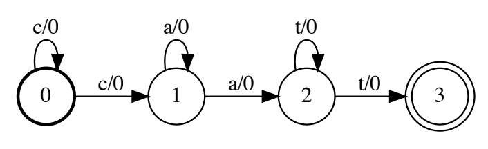
Figure 1: Alignment graph

This graph is sometimes called weighted finite state acceptor (WFSA). The bold state marked 0 at the beginning is a start state, the concentric circle marked 3 is an accepting state. On each edge, there’re a label and a weight on both sides of a slash. Any path in this graph is an encoding of an alignment.

Problem: too many alignments

There’s a problem when using all of the alignments. The $\mX$ input audio can have lots of frames, in practice they can be as high as thousands. The $\mY$ transcription can have lots of letters, in practice it can be hundreds or more. This is an astronomically large number of alignments, so we can’t compute individual score and sum all of them.

Solution: the forward algorithm(dynamic programming)

Define forward variable $\alpha_t^u$, the subscript $t$ is where we are in the input and the superscript $u$ is where we are in the output. This represents the score for all alignments of length $t$ which end in the output $y_u$.

Suppose $\mX=[x_1,x_2,x_3,x_4]$, $\mY=[c,a,t]$, the forward variable $\alpha_2^c$ represents the score of all possible alignments of length two up to the first two frames that ends in $c$ in the first output of the transcription. There’s only one possible alignment for that $x_1\rightarrow c$, $x_2\rightarrow c$. This is simple to compute.

Similarly, $\alpha_2^a$ has only one possibility.

For $\alpha_3^a$, there are two possible alignments

• $A_1$: $x_1\rightarrow c$, $x_2\rightarrow c$, $x_3\rightarrow a$
• $A_2$: $x_1\rightarrow c$, $x_2\rightarrow a$, $x_3\rightarrow a$

This is the naive approach to compute $\alpha_3^a$.

Using this forward variable, we seek to model the probability distribution $P(\mY \mid \mX) = \sum_{a \in A} P(a)$, where $A$ is the set of all possible alignments from $\mY$ to $\mX$. This decomposes as

where $P(a_t \mid \mX)$ are the output logits of a system such as an RNN. That is, to compute the likelihood of the transcript $\mY$ we must marginalize over an intractably large number of alignments. We may do this with a recursive decomposition of the forward variable. The below presentation is inspired by https://distill.pub/2017/ctc/, which is an excellent introduction to the algorithm.

First, we permit an alignment to contain the empty output $\epsilon$ in order to account for the fact that audio sequences are longer than their corresponding transcripts. We also collapse repetitions, so that ${a, \epsilon, a, a, \epsilon, a}$ corresponds to the sequence $aaa$. We will also define $\alpha$ using an alternative transcript $Z$, which is equal to $\mY$ but is interspersed with $\epsilon$. That is, $Z = {\epsilon, y_1, \epsilon, y_2, …, y_n, \epsilon }$.

Now, suppose $y_i = y_{i+1}$, so that $Z$ contains a subsequence $y_i, \epsilon, y_{i+1}$, and suppose $y_{i+1}$ occurs at psosition $s$ in $Z$. Then the alignment for $\alpha_{s}^t$ can be arrived at by one of two ways: either the prediction at time $t-1$ can be $y_{i+1}$ (in which case the repetition is collapsed) or else the prediction at time $t-1$ can be epsilon. So, we may decompose:

where the elements of the sum represent the two possible prefixes to the alignment. If, on the other hand, we have $y_i \ne y_{i+1}$ then there is the additional third possibility that the prediction at time $t-1$ is equal to $y_i$. So, we have the decomposition

By computing $\alpha_{\vert Z\vert}^{T}$, we may effectively marginalize over all possible alignments between the transcript $\mY$ and the audio $\mX$, allowing efficient training and inference. This is called Connectionist Temporal Classification, or CTC.