Self Supervised Learning in Computer Vision

The current focus in Computer Vision lies in learning of visual representation from supervised data and using these representations/model weights as initializations for other tasks which lack availability of labelled data. Labelling data can be expensive, for instance, the Imagenet dataset has ~14 million images and 22,000 categories taking ~22 human years to label.

Pretext Task

The pretext task is a self-supervised learning task solved to learn visual representations, with the aim of using the learned representations or model weights obtained in the process, for other downstream tasks. The pretext task is usually performed on a property that is inherent in the dataset itself.

Popular pretext tasks for images:

1. Predicting relative position of patches within an image
2. Predicting permutation type of image patches (Jigsaw Puzzles)
3. Predicting the kind of rotation applied

What is missing from pretext tasks?

There is a fairly big mismatch between what is being solved in the pretext tasks and what needs to be achieved by the transfer tasks. Thus, the pre-training is not suitable for final tasks. Performance at each layer can be assessed (using linear classifiers) to figure out which layer’s features to use for the transfer tasks.

Pre-trained features should satisfy two fundamental properties:

1. Must represent how images relate to one another
2. Be robust to nuisance factors

Popular method for self-supervised learning

A popular and common method for self supervised learning is to learn features that are robust to data augmentation. Learn features such that,

Features produced by the network for an image should be stable under different types of data augmentation techniques. This property is extremely useful because the features are going to be invariant to the nuisance factors.

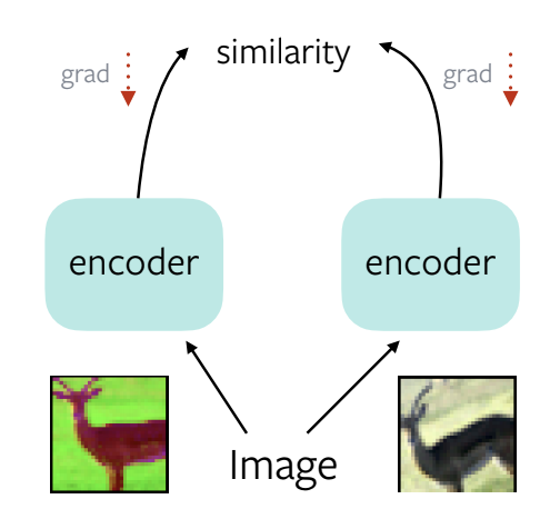
Figure 1: A trivial solution to learning self-supervised representations

Take an image, apply two different data augmentations to it, feed it through encoder, compute the similarity. Get the gradients and backpropagate. The network then learns to produce a constant representation for both augmentations.

Trivial Solution: Produce the same features for all input images. The representations collapse and become unusable for downstream recognition tasks.

Categorization of recent self-supervised methods:

1. Maximize Similarity Objective
2. Redundancy Reduction Objective

For evaluation, a subset of the Imagenet dataset (1.3 million images over 1000 categories) without labels is used to pre-train a randomly initialized Resnet-50 model.

What are the different ways to perform transfer learning and evaluate its performance?

We can do one of 2 things:

1. Linear classifier on top of fixed features output by the network (For classification tasks)
2. Finetune the entire pretrained network on the target task (For detection tasks)

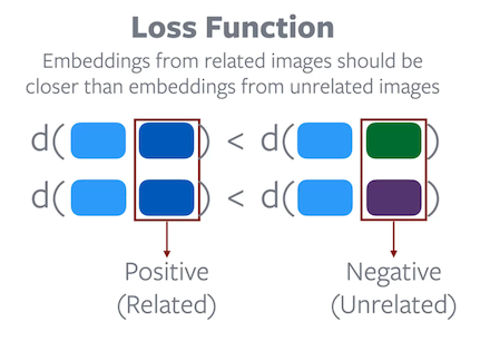
Contrastive Learning

Loss function: Embeddings from related images should be closer than embeddings from unrelated images.

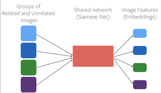
Figure 2: The use of a base encoder in Contrastive Learning

Different Contrastive Learning methods include:

1. Pretext-Invariant Representation Learning (PIRL)
2. SimCLR
3. MoCo

Pretext-Invariant Representation Learning (PIRL)

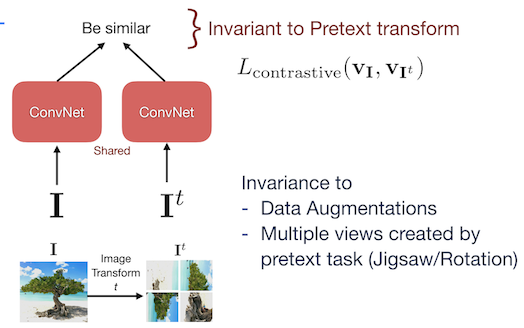
Figure 3: Architecture of PIRL

An image $I$ and its augmentation $I^t$ is passed through the network and the contrastive learning loss is applied in such a way that the network becomes invariant to the pretext task. The aim is to achieve high similarity for image and patch features belonging to the same image. And low similarity for features from other random images. The pretext task of PIRL tries to achieve invariance over data augmentations rather than predicting the data augmentation.

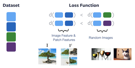
Figure 4: Loss function of PIRL

Semantic Features

Figure 5: Performance of pretraining using PIRL vs Jigsaw at each layer

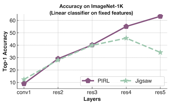
• A linear classifier is used at each layer to probe and compute the accuracy. One is trained using PIRL and other using Jigsaw.
• Jigsaw is trying to predict the permutation, whereas PIRL is trying to be invariant to it.
• Performance for PIRL keeps increasing indicating that the feature is becoming increasingly aligned to the downstream classification tasks.
• Jigsaw is trying to retain pretext information, the performance plateaues and then drops down sharply and it ends up not performing well for the transfer tasks.

Sampling Positives and Negatives

There are many ways to obtain samples that make up related (positive) and unrelated (negative) pairs:

1. Crops of an image: Contrastive Predictive Coding (CPC) based models use patches from one image that are close-by as positives (related) and patches that are far-away from each other as negatives (unrelated).

2. Crops across images: Patches from within one image are considered related and patches from 2 different images are considered unrelated. Used in MoCo and SimCLR

3. Videos: Frames that are closeby in temporal space are related, and those far-away are unrelated

4. Multimodal - Video and Audio: Video sequences along with their corresponding audio are related. Video sequences from one video and audio from another are unrelated.

5. Video Object Tracking: An object is tracked through multiple frames in a video. Detection patches from the same video are related. Detection patches from different videos are unrelated.

What is the fundamental property of Contrastive Learning that prevents trivial solutions?

Figure 6: Loss function of Contrastive Learning

The objective function of Contrastive Learning is designed to prevent trivial solutions. The aim of the function is to make sure the distance between positive embedding pairs are smaller than the distance between negative embedding pairs. Hence, a trivial solution, where a constant distance is assigned to all embedding pairs, is impossible to attain through a minimization process on the given objective function. However, research has shown that good negative pairs are crucial for Contrastive Learning to work well.

SimCLR

In SimCLR, Simple Framework for Contrastive Learning of Visual Representations, two correlated views of an image are created using augmentations like random cropping, resize, color distortions and Gaussian blur. A base encoder is used along with a projection head to obtain representations that are used to perform contrastive learning.

It utilizes a large batch size to generate negative samples. The batch can be spread across multiple GPUs independently. Images from one GPU could be considered as negatives for those from another GPU.

Advantages of SimCLR:

1. Simple to implement

Disadvantages of SimCLR:

1. Large batch size required
2. Large number of GPUs required

How do we solve the compute problem in the SimcLR?

A Memory bank can be used to maintain a momentum of activations across all features. With each forward pass of an image, the memory bank features are updated using the new embeddings. These memory bank features can then be used as negatives for contrastive loss.

Advantages of Memory bank:

• Compute efficient. Requires one Forward Pass to compute the embeddings.

Drawbacks of Memory bank:

• Not online. Features become stale very fast.
• Requires large amount of GPU RAM.
• Hard to scale storage to millions of images.

MoCo

MoCo, or, Momentum Contrast, is a contrastive method that utilizes a memory bank to maintain a momentum of activations. It works by using 2 encoders. The $f_{\vtheta}$ encoder is the encoder that needs to be learnt. $f_{\vtheta_{\text{EMA}}}$ encoder maintains an exponential moving average of $f_{\vtheta}$.

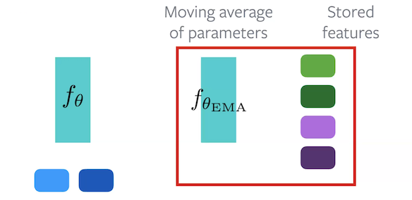
Figure 7: Architecture of MoCo

During Forward Pass, each sample is forwarded through both encoders. Some of the embeddings from $f_{\vtheta_{\text{EMA}}}$ are kept aside for use as negative embeddings. For the algorithm, original embeddings comes from $f_{\vtheta}$, positive embeddings from $f_{\vtheta_{\text{EMA}}}$ and negative embeddings come from the set of stored embeddings.

Advantages of MoCo:

• Can easily be scaled in terms of memory usage as the full dataset need not be stored.
• Is an online solution, as the moving average is continuously updated.

Drawbacks of MoCo:

• Two Forward Passes are required, one through $f_{\vtheta}$ and another through $f_{\vtheta_{\text{EMA}}}$.
• Extra memory required for parameters/stored features.

Clustering methods

How CL and clustering are related to one another?

In Constrastive Learning, each sample has corresponding positives and negatives, and the aim of the learning task is to try and bring together positive embeddings, while pushing apart negative embeddings. Essentially we are creating groups within the feature space.

Clustering, on the other hand, is a more direct way to achieve grouping, as it naturally creates groups in the feature space.

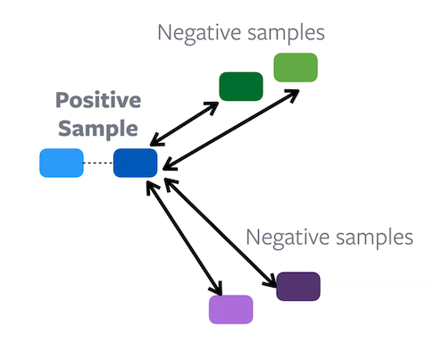
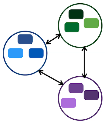
Figure 8: Difference between Contrastive learning (Left) and Clustering (Right)

SwAV

The SwAV (Swapping Assignments between Views) algorithm is an online clustering method. The idea here is to maximize the similarity of a given image $I$ and augmentation of that image $\text{augment}(I)$ and, in doing so, ensure they belong to the same cluster.

Samples and their augmentations are represented by different shades of the same color. The similarity of each sample’s embedding with each of the prototypes (cluster-centers) is computed. The sample is then assigned to the prototype with the highest similarity. The aim of the network is to assign an image and its augmentation to the same prototype.

Can it lead to any trivial solution?

A trivial solution is possible where every sample is assigned to the same group/cluster/prototype. This would cause a collapsed representation for any given input.

How to avoid trivial solution?

1. Equipartition constraint

   
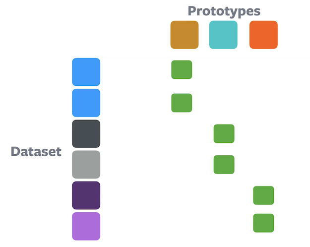
   Figure 9: Clustering using an equipartition constraint

   Given n samples and k partitions, each cluster is allowed to have a maximum of n/k samples. Embeddings are equally partitioned and this prevents the single cluster trivial solution. Optimal-transport based clustering methods such as the Sinkhorn-Knopp algorithm inherently guarantees the constraint.

2. Soft assignment

   
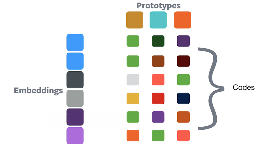
   Figure 10: Clustering using soft assignment

   In soft assignment, a sample belongs to all prototypes with some proportion of each, such that they all sum up to 1.0. The composition values can be treated as a code that indicates how each embedding is encoded in the ‘prototype’ space.

Consider the case where we have a high class imbalance. If we use the equipartition method, then won’t that give inacurate results?

Soft assignment solves this problem by representing a lot more classes (logically) than hard assignment. It gives a richer representation and is less sensitive to $k$ (number of classes) and hence $k/n$. However, if hard assignment is used, the class imbalance and the fixed value of $n/k$ will create inaccuracies.

Training SwAV:

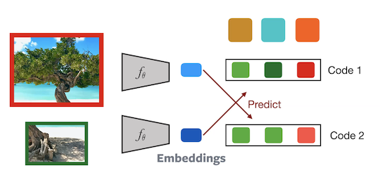
Figure 11: Architecture of SwAV

2 crops from an image are passed through the network to compute the corresponding codes. The $2^{\text{nd}}$ code is then predicted from the $1^{\text{st}}$ embedding and vice versa. This task forces the network to become invariant to data augmentations. Gradients are backpropagated onto the prototypes as well. Hence this model is updated in an online manner.

Advantages of SwAV:

1. No explicit negatives needed
2. Optimal transport methods avoid trivial solutions.
3. Faster convergence than contrastive learning.
   • The code space imposes more constraints and the embeddings are not directly compared.
4. Less compute requirements.
5. Smaller number (4-8) of GPUs required.

Pretraining on ImageNet without labels:

Even though ImageNet without labels can be used for self supervised learning, there is an inherent bias in the dataset due to the curation/hand-selection process involved.

1. Images belong to 1000 specific classes
2. Images contain a prominent object
3. Images have very limited clutter and very few background concepts

Pretraining on Non-ImageNet data

Pretraining on Non-ImageNet data hurts performance.

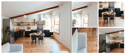
Figure 12: Example of a problematic image from a non-imagenet dataset

Consider the above image. One crop has a refrigerator and the other crop could be that of a table/chair. The algorithm would try to create similar embeddings for both of them, because they belong to the same image. This is not what we expect from the training process.

Real world data has very different distributions. They may sometimes even be cartoon images or memes, and there is no guarantee that an image will contain a single (or sometimes, any) prominent object.